Microsoft Excel

Fix Blanks in Excel Data with GO TO SPECIAL and the COPILOT Function

Every serious Excel user should have Go To Special in their toolkit. It is one of the fastest ways to find blanks, formulas, constants, or other specific cell types in a worksheet — and it pairs beautifully with the new Excel COPILOT function when your data needs more than a quick formula can handle.

In this tutorial I'll walk you through a practical exercise. We'll count blanks with COUNTIF, highlight them with Go To Special, delete the rows that contain them, then tackle a real-world address problem two different ways: with a 3D reference combined with Go To Special, and with the Excel COPILOT function.

Count blanks with COUNTIF

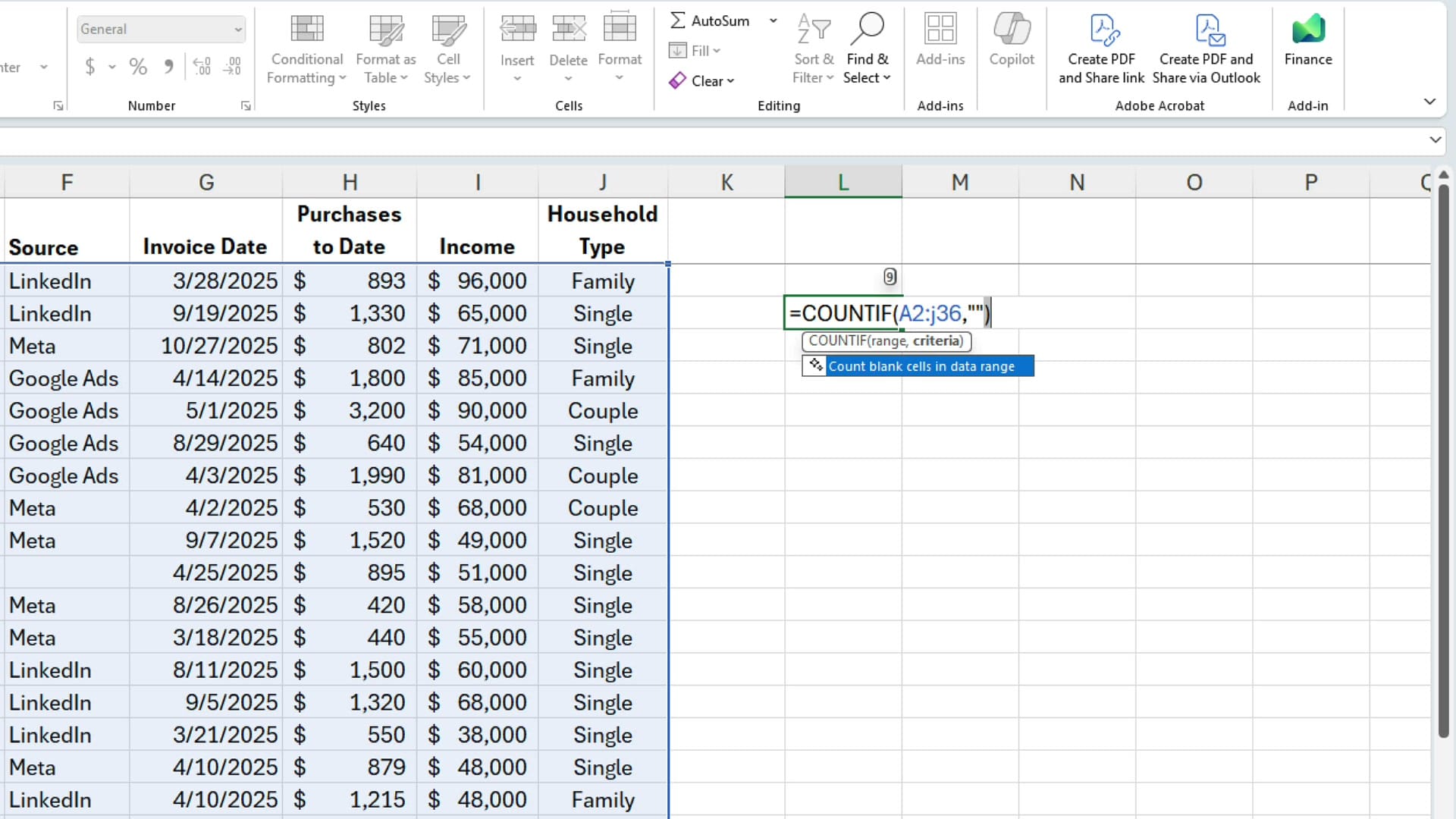
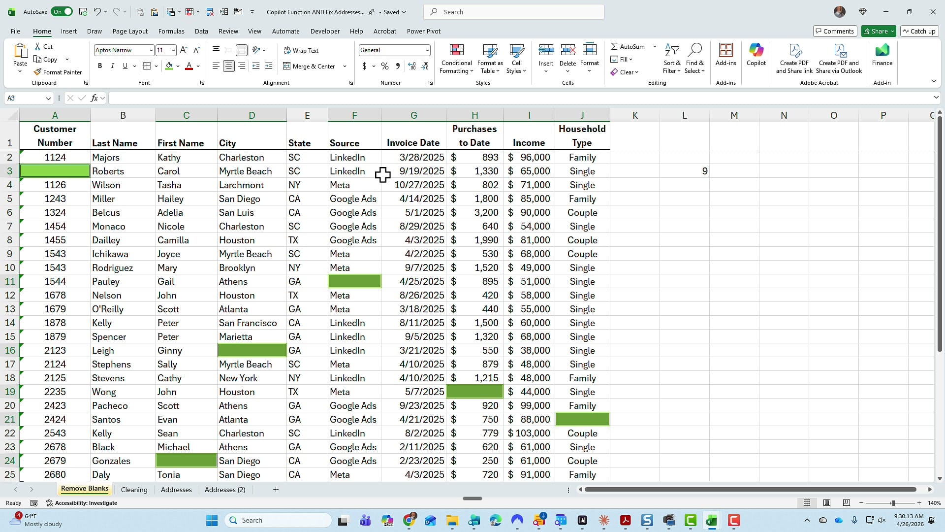
I have a range of customer data from A2 to J36 — a regular range, not a formatted Excel table (it doesn't matter for this exercise either way). Notice cell A3 is blank, and so is cell F11. Before doing anything else, I want to know exactly how many blank cells the range contains.

That's a one-line formula:

=COUNTIF(A2:J36,"")

The empty quotes tell COUNTIF to count cells with no value. The result: nine blanks across the worksheet.

Excel COUNTIF formula counting blank cells in a customer data range — =COUNTIF(A2:J36,"") returns 9 — the number of blank cells in the range. The ScreenTip even says "Count blank cells in data range."

Highlight blank cells with Go To Special

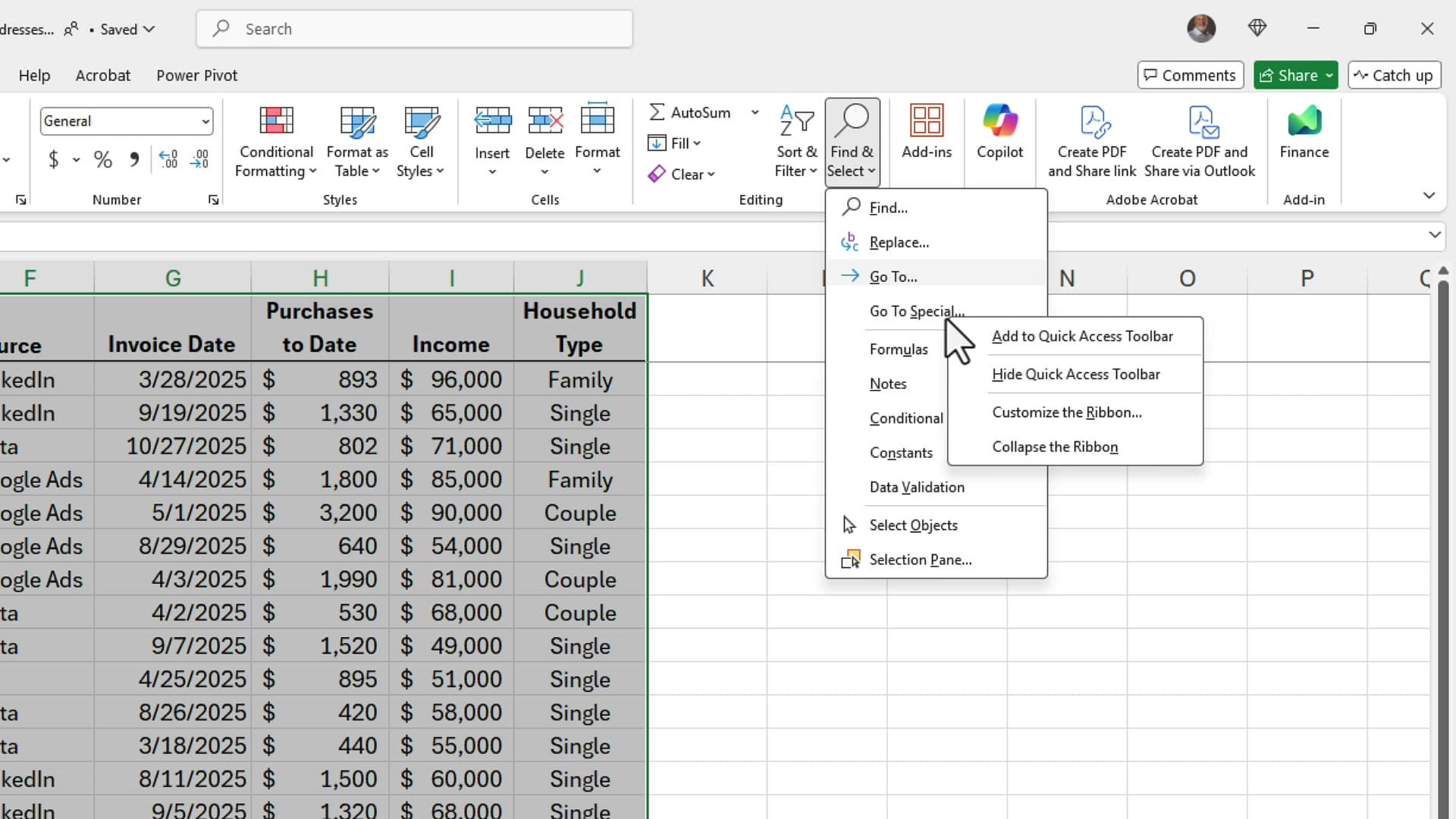
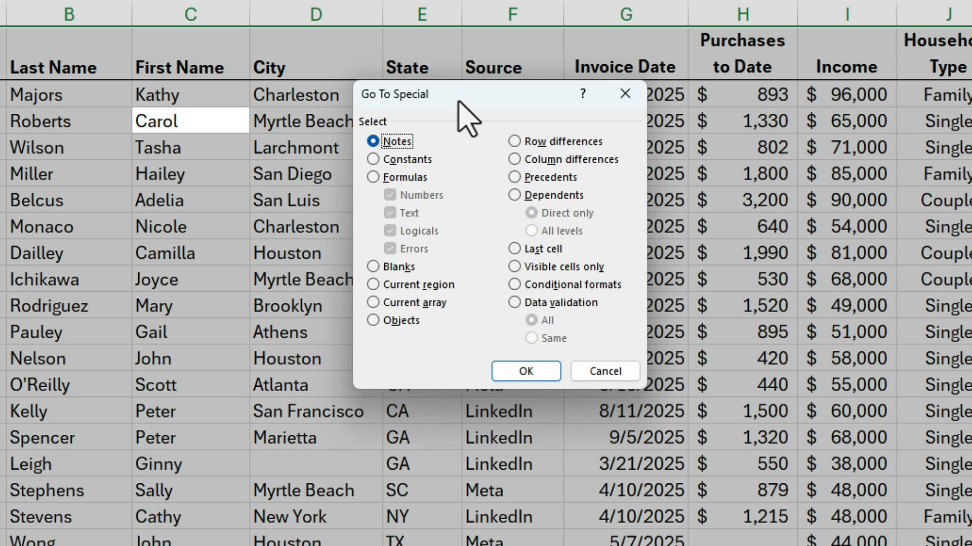
Now I want to put a yellow background on every blank cell so they stand out. Click anywhere in the data, press Ctrl + A to select the whole range, then open Go To Special.

With the mouse, that's on the Home tab → Find & Select → Go To Special. While you're there, right-click Go To Special and add it to your Quick Access Toolbar — you'll use it constantly.

Find and Select dropdown showing Go To Special with right-click option to add it to the Quick Access Toolbar — Home → Find & Select → Go To Special. Right-click it to pin it to your Quick Access Toolbar.

In the Go To Special dialog, choose Blanks and click OK. Excel selects every blank cell in the range — including A3 and F11 — in one step. Apply a yellow fill from the Home tab and your blanks light up immediately.

Excel Go To Special dialog box with the Blanks option selected — The Go To Special dialog. Pick Blanks and click OK to select every empty cell in the range at once.

Excel data range with all nine blank cells highlighted in green to make them visible — All nine blanks are now highlighted, scattered across different columns and rows.

Delete rows that contain blanks

Highlighting is useful, but a viewer recently asked a follow-up: "If a row has a blank in it, I want to delete the entire row. Can that be done?" Absolutely.

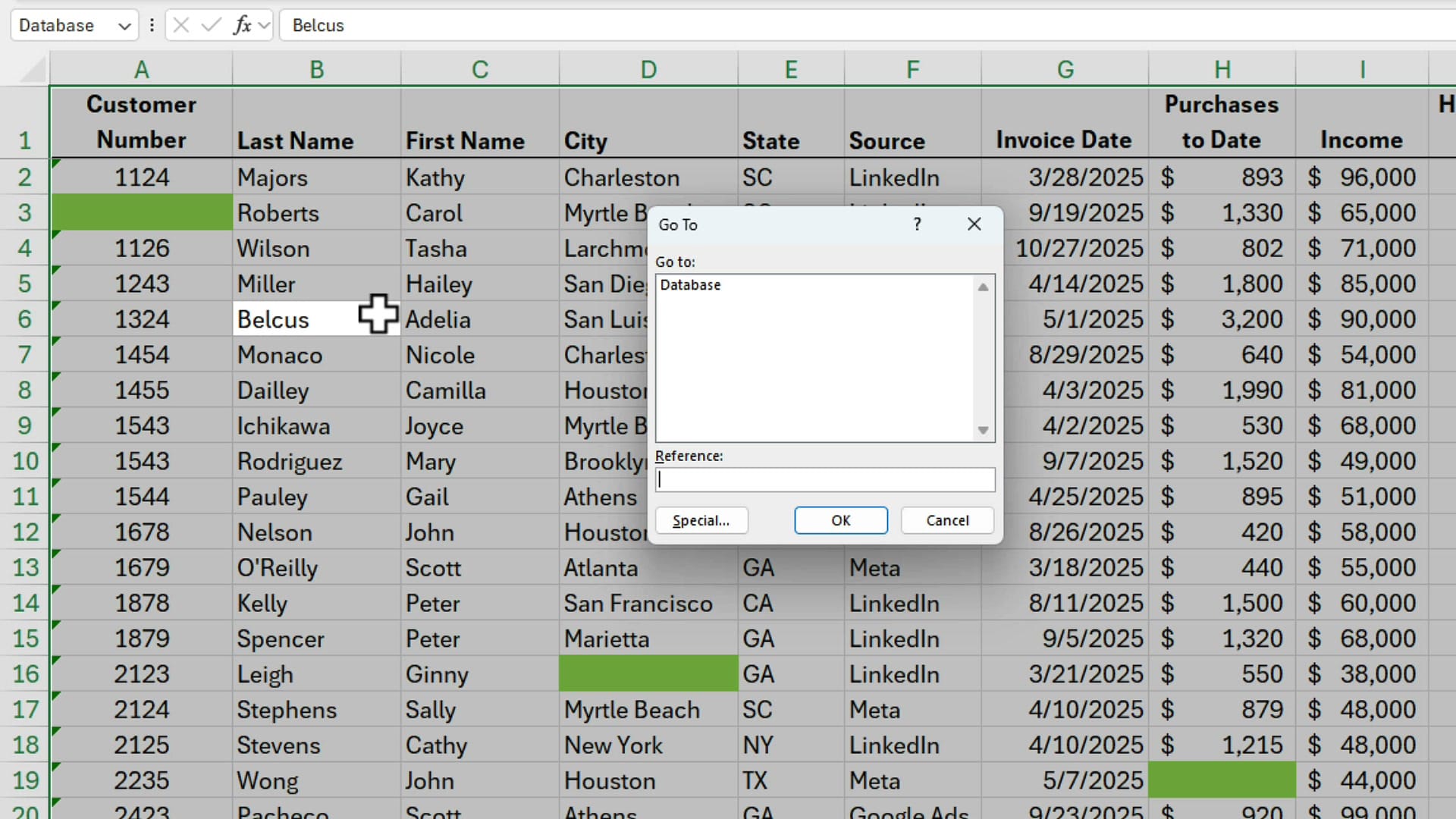
The steps are nearly identical. Click in the data, press Ctrl + A to select all, then press Ctrl + G (or F5) to open the Go To dialog. Click the Special... button at the bottom-left, choose Blanks, and click OK.

Excel Go To dialog box opened with Ctrl+G showing the Special button at the bottom-left — Ctrl + G (or F5) opens the Go To dialog. Click Special... to jump into Go To Special.

With every blank selected, right-click any of them and choose Delete. In the Delete dialog, pick Entire row and click OK.

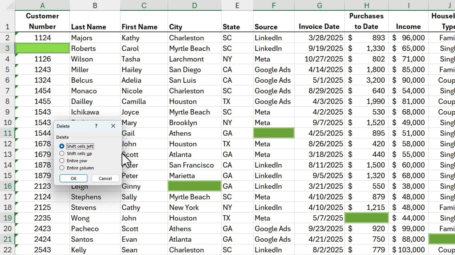
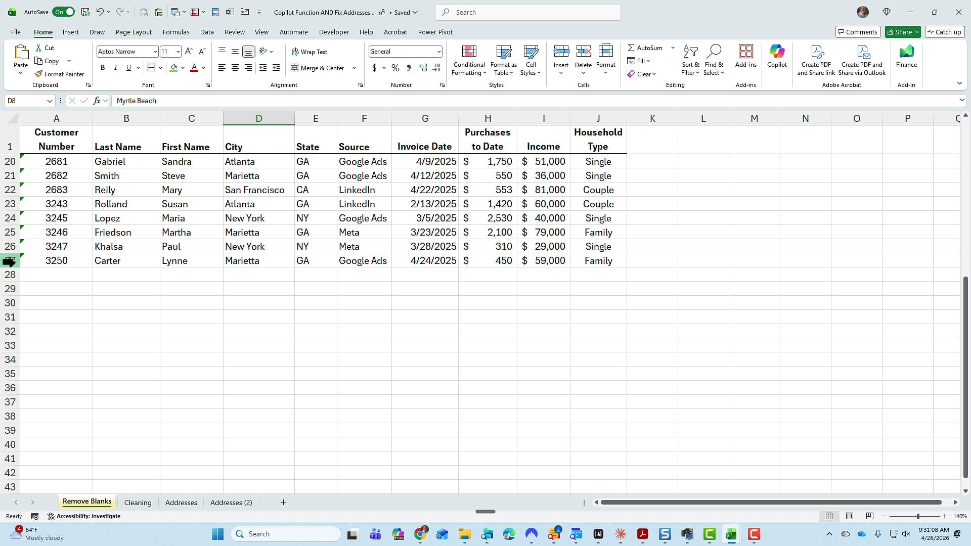
Excel Delete dialog box with Entire row option selected — Choose Entire row to remove every record that contained a blank cell.

The math checks out: I started with 36 rows, deleted 9, and ended up with 27. The COUNTIF formula that previously returned 9 now returns 0.

Excel worksheet after deleting all rows that contained blanks, leaving 27 clean records — Clean dataset — 27 complete records remain after deleting all rows with blanks.

The vertical address problem

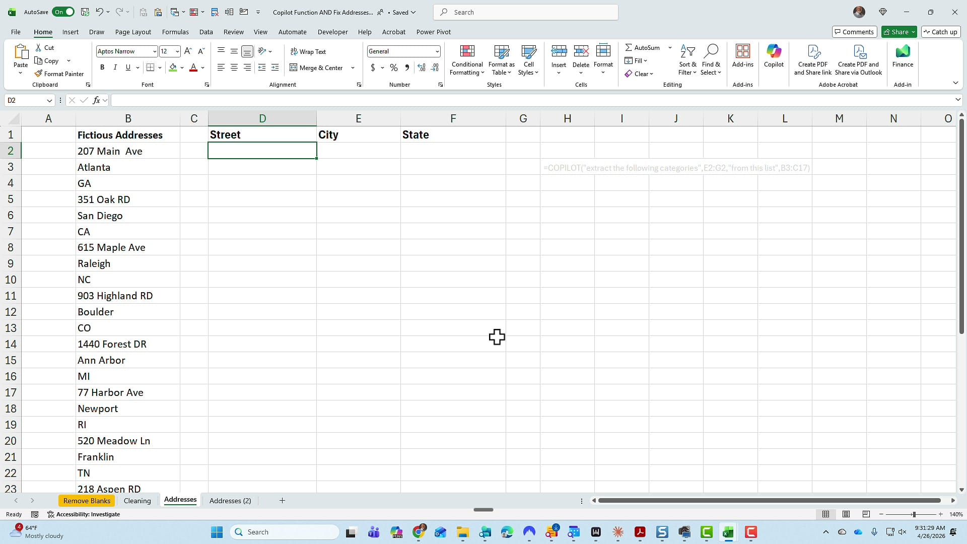
Switching worksheets, I have a different challenge. Cell B2 is a street address, B3 is the city, and B4 is the state. The data is running vertically when it needs to run horizontally — into Street, City, and State columns at D1:F1.

I'll show you two ways to fix it. First with a 3D reference and Go To Special, then with the COPILOT function. One important note before we start: every record in this list is consistent — three items per address (street, city, state) with no extra suite numbers thrown in. That consistency is what makes the first method work.

Excel worksheet with addresses stacked vertically in column B and empty Street, City, State columns at D, E, and F — The starting layout: addresses run top-to-bottom in column B, but I need them flowing left-to-right into D, E, and F.

Fix addresses with 3D reference and Go To Special

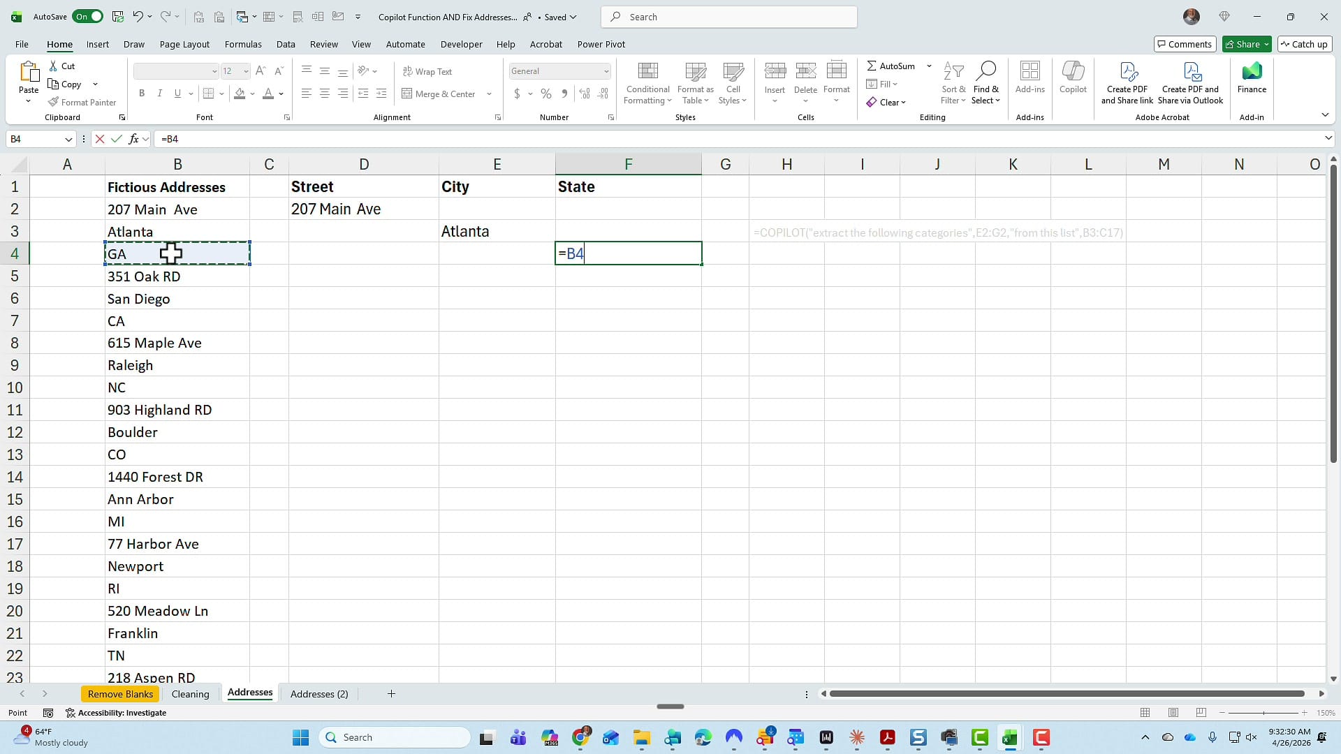
In cell D2, type =B2 for the street. In E2, =B3 for the city. In F2, =B4 for the state. Then highlight D2:F2 and autofill down to the bottom of your data.

Excel cell F2 showing the formula equals B4 for the state, building a 3D reference to pull addresses horizontally — Build the 3D reference: D2 = B2 (street), E2 = B3 (city), F2 = B4 (state). Then autofill down.

The autofill creates a pattern that pulls every third cell — but it also produces lots of blanks because the pattern hits empty cells in column B too. With the new range still selected, open Go To Special and pick Blanks.

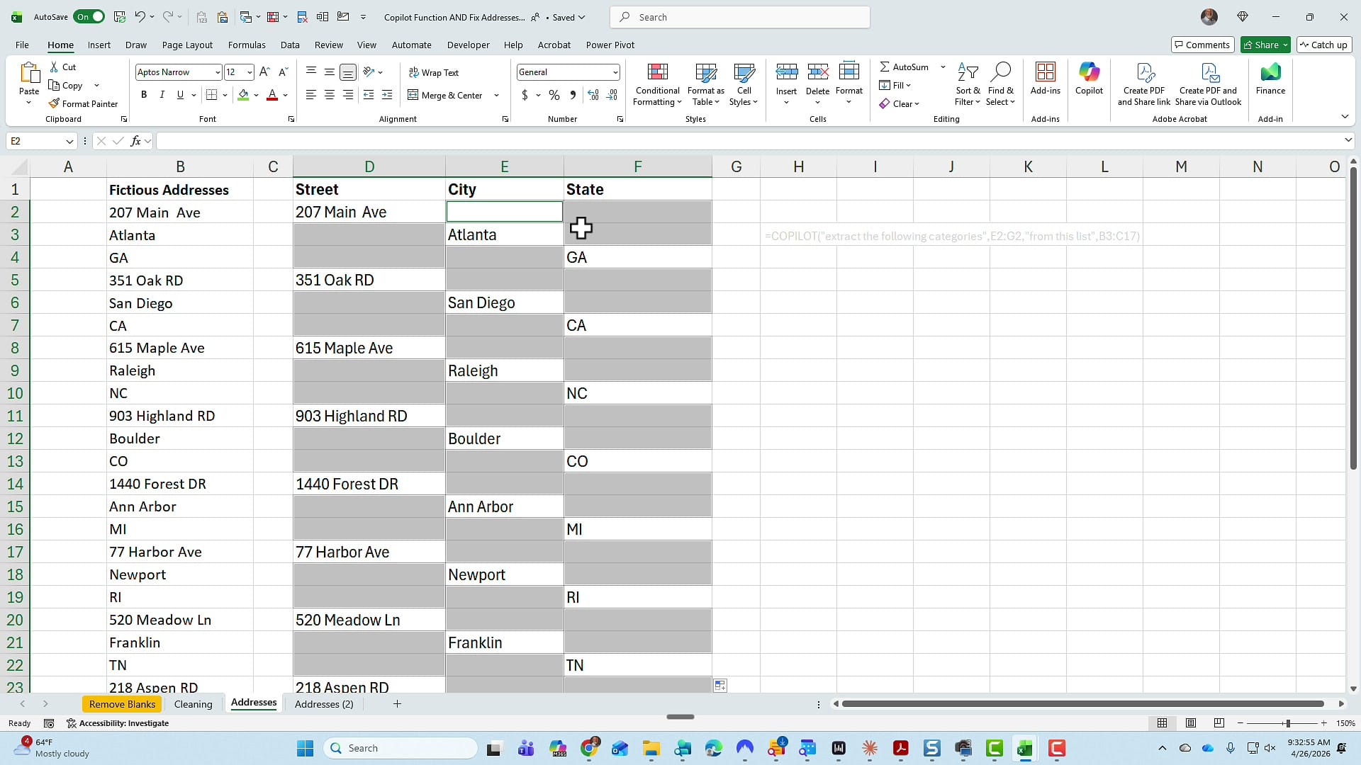
Excel showing the autofilled 3D reference with all the in-between blank cells selected and highlighted — After autofill, every other row produces a blank. Go To Special → Blanks selects them all at once.

Right-click and choose Delete. This time, do NOT pick Entire row — that would wipe out neighboring data. Pick Shift cells up instead. The remaining cells collapse upward and you're left with a clean horizontal address list.

Excel worksheet showing addresses now arranged horizontally in Street, City, and State columns after the shift cells up operation — Shift cells up collapses the blanks and leaves you with a tidy horizontal address list.

One last cleanup: the cells still contain the 3D reference formulas, which point back to column B. To freeze the values in place, highlight the new data, drag-and-drop with the right mouse button, drop it back where it was, and choose Copy here as values only. That's faster than the standard Copy → Paste Special → Values workflow.

Extract addresses with the COPILOT function

That 3D reference works, but my preferred method is the new Excel COPILOT function. It's one of my favorite features in Excel right now. You will need a paid Microsoft Copilot license — Microsoft now calls it a premium license — to use it.

The syntax for this exercise looks like this:

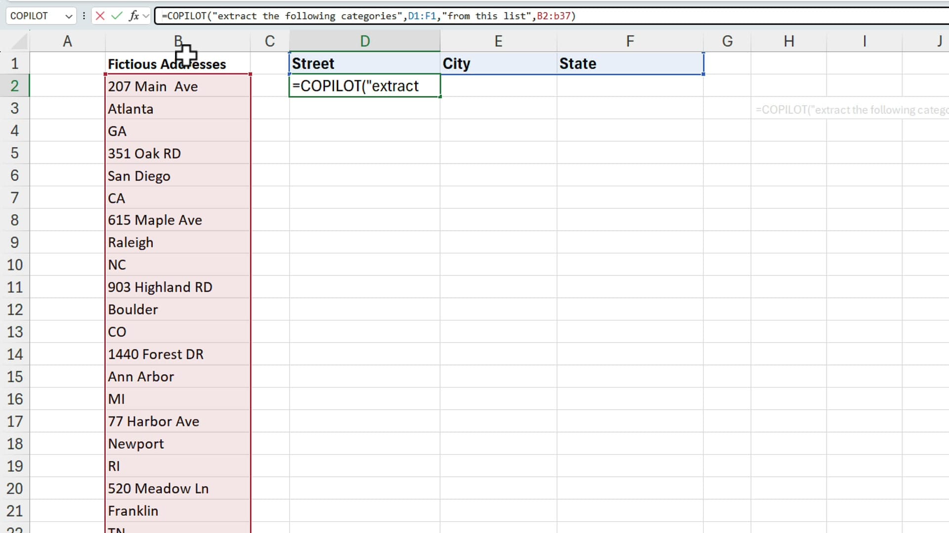
=COPILOT("extract the following categories",D1:F1,"from this list",B2:B37)

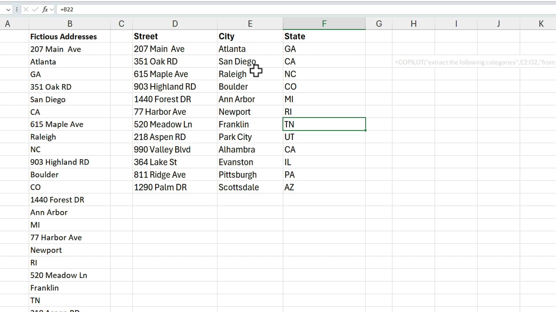
You're telling Copilot to extract the categories you defined in your headers (Street, City, State at D1:F1) from the address list (B2:B37). One formula, no autofill, no Go To Special, no shifting cells up.

Excel formula bar showing the COPILOT function syntax extracting categories from a list of addresses — The COPILOT function syntax: a description, the categories range, a connecting phrase, and the source list.

Press Enter and give it a second. Copilot reads each address in column B, identifies the street, city, and state, and drops them into the right columns.

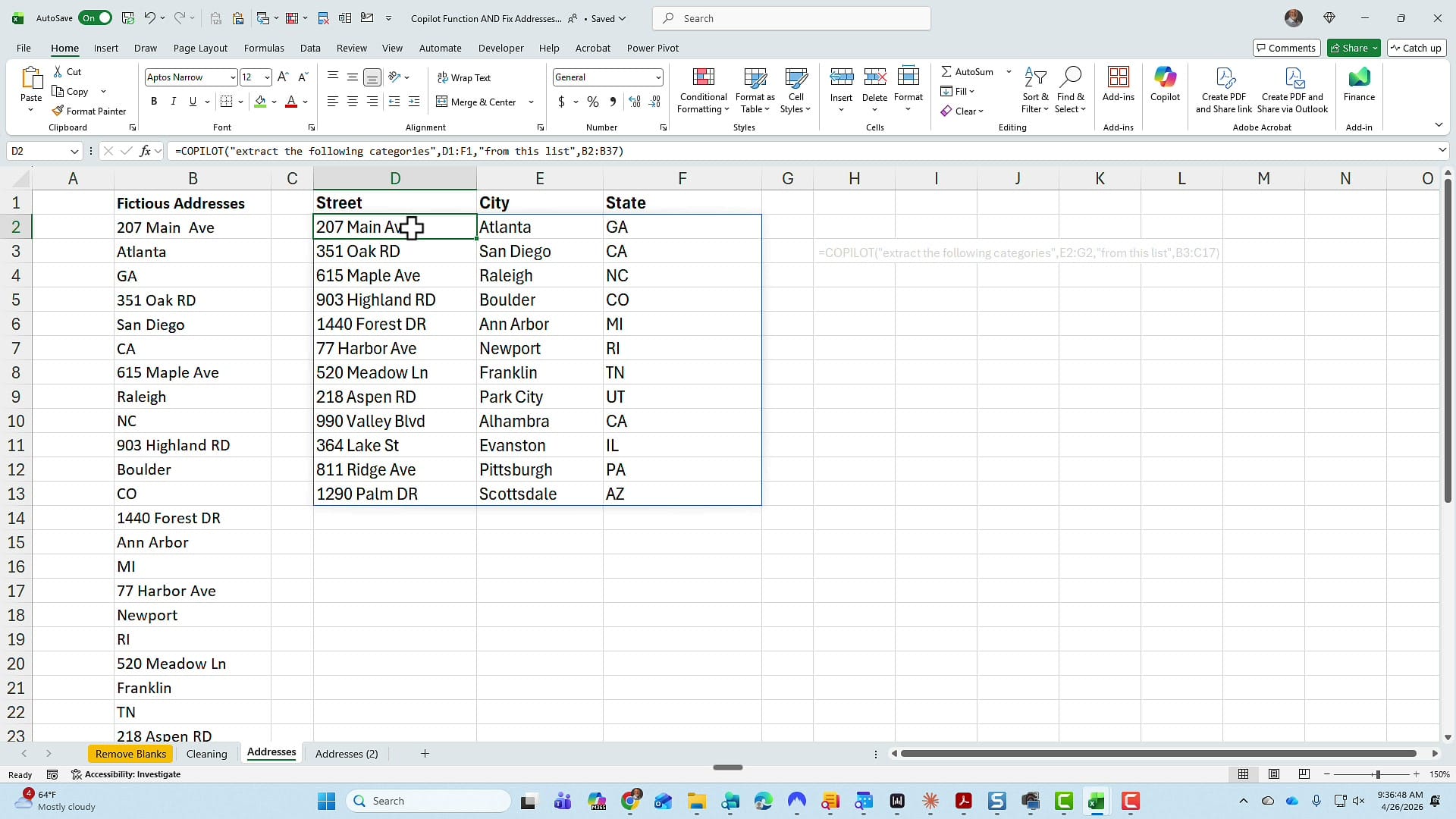
Excel worksheet with addresses fully extracted into Street, City, and State columns by the COPILOT function — The COPILOT function fills the Street, City, and State columns in one go. Always sanity-check the last row — here, 1290 Palm DR, Scottsdale, AZ is correct.

Always go check the result. The last record should be Arizona, 1290 Palm Drive — and it is. To freeze the values in place, do a copy / paste values just like before.

Handle inconsistent addresses with COPILOT

Here's where the COPILOT function shines. On a different worksheet, the addresses are not consistent anymore — some include suite numbers, others don't. The 3D reference approach falls apart immediately because the pattern of three items per record is broken.

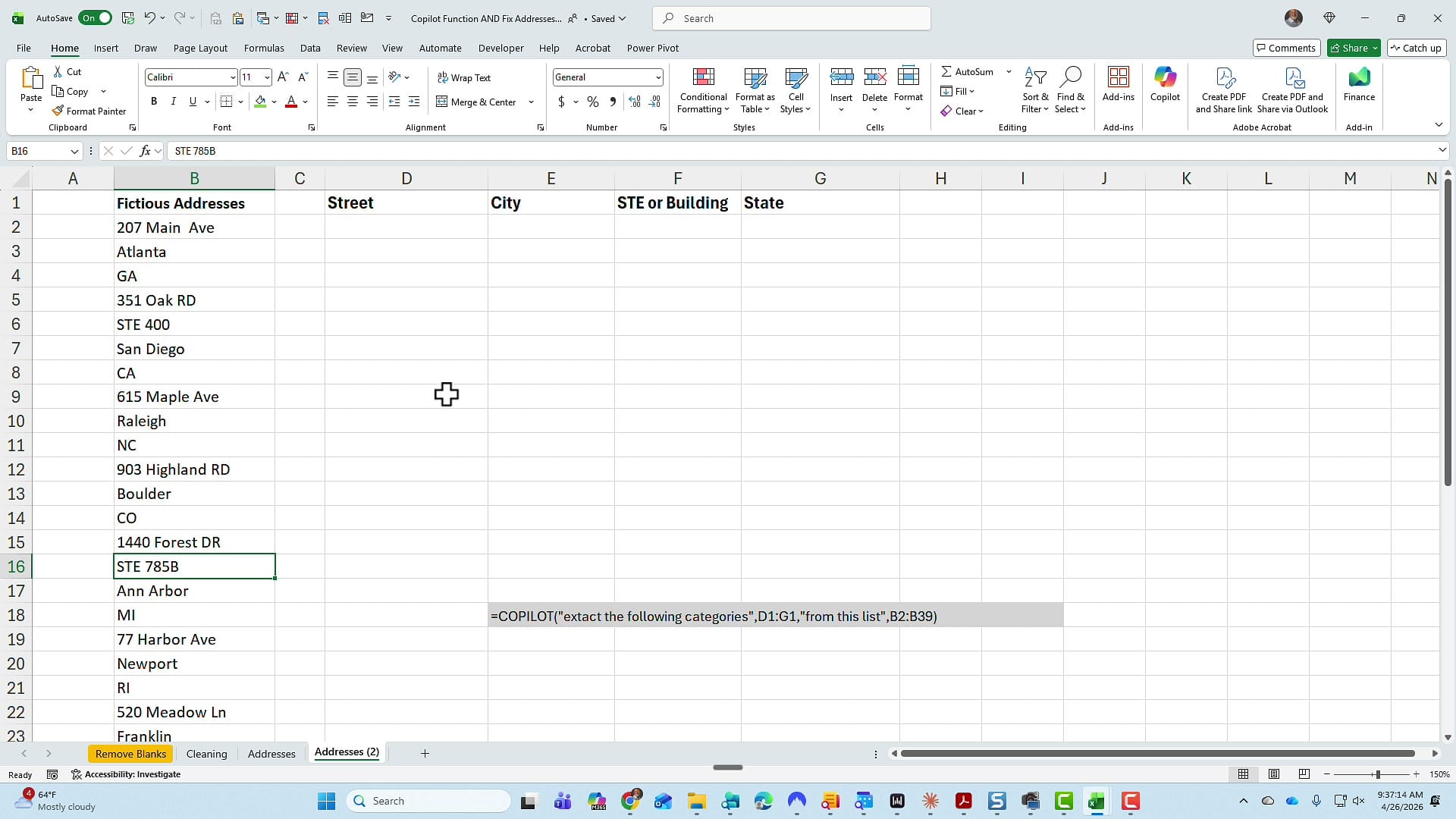
Excel worksheet with inconsistent address data including suite numbers like STE 400 and STE 785B mixed in — Some records have suite numbers (STE 400, STE 785B), others don't. The 3D reference can't handle this.

I just add an extra column header — STE or Building — so my categories now run from D1 to G1. The formula becomes:

=COPILOT("extract the following categories",D1:G1,"from this list",B2:B39)

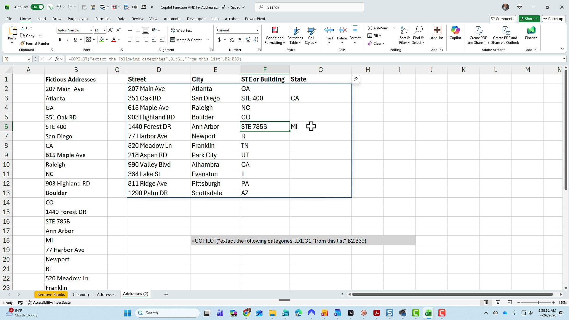
Excel COPILOT function correctly extracting addresses with mixed suite numbers into separate Street, City, STE or Building, and State columns — COPILOT handles the inconsistency cleanly: 351 Oak RD goes to Street, San Diego to City, STE 400 to STE or Building, CA to State.

Take a look at the second record — 351 Oak Drive, Suite 400, San Diego, California. The suite number lands in its own column. The third record has no suite, so that column stays blank for that row. The COPILOT function understood the structure of each address individually, no extra setup required.

When to use each method

Counting and highlighting blanks — COUNTIF + Go To Special. Fast, free, no AI required.
Deleting rows with blanks — Go To Special → Blanks → right-click → Delete → Entire row.
Reorganizing perfectly consistent data — 3D reference + Go To Special + shift cells up. No license needed.
Reorganizing inconsistent data — COPILOT function. Requires a paid Copilot license but handles real-world messiness without breaking.

If you don't have a Copilot license yet, the Go To Special workflow is a powerful tool on its own. If you do have one, the COPILOT function turns what used to be a multi-step cleanup into a single formula.