Microsoft Excel

Excel Conditional Formatting: Highlight Rows Where Spend Goes Over Budget

Use a formula-based conditional formatting rule with a mixed reference to highlight every row where the spend column exceeds the budget column.

A subscriber sent me a spreadsheet with a budget column and an actual-spend column, and asked how to highlight the entire row whenever the spend went over the budget. It is a classic conditional formatting with a formula problem, and once you understand the dollar signs, you can reuse this technique for dozens of similar reports.

I will walk through it in Excel for the web, but every step works identically in Excel desktop — the menu lives on the Home tab in both versions.

The data set

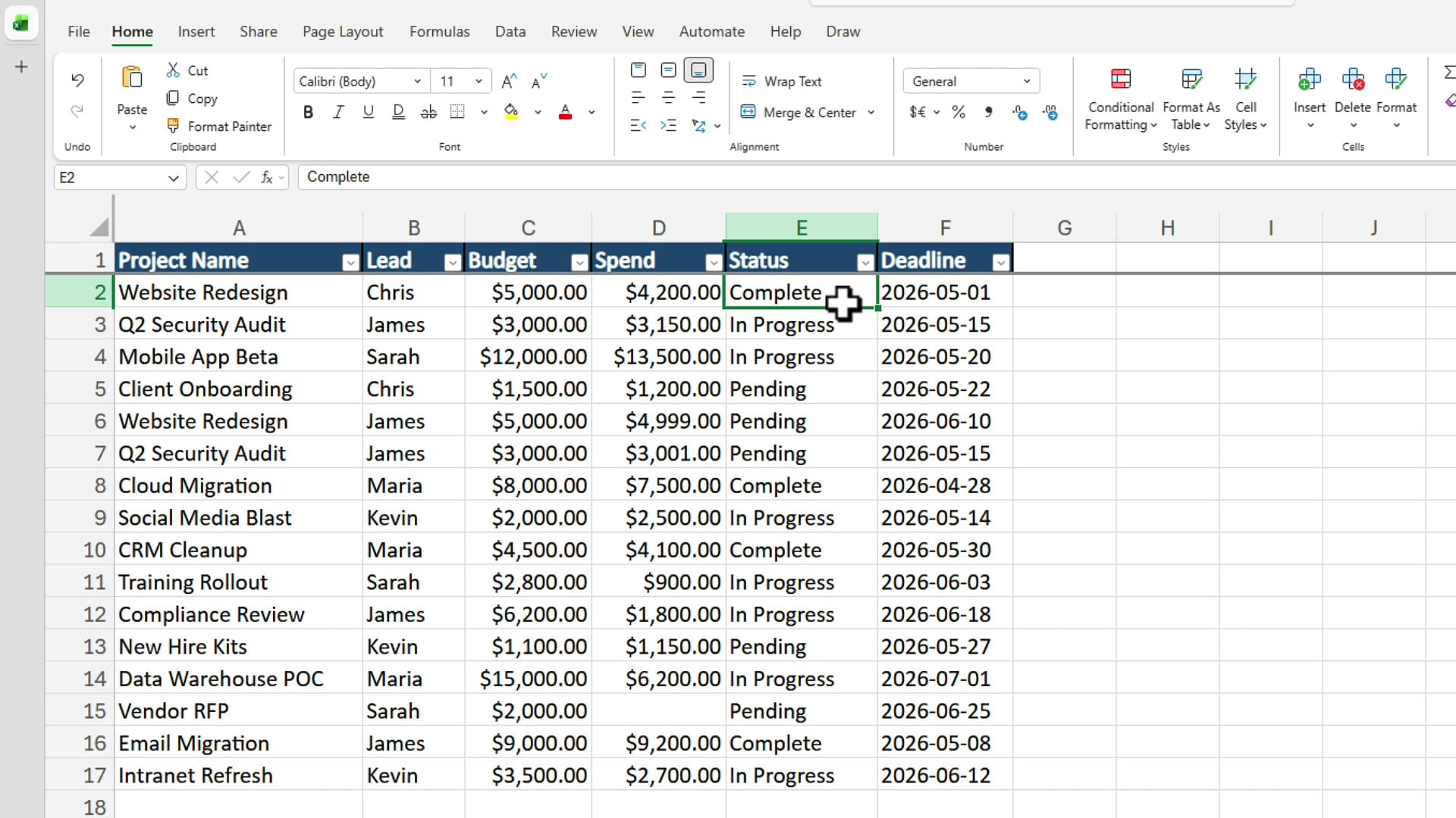
Excel spreadsheet showing project budget and spend columns with rows for each project — The starting data: Budget in column C, Spend in column D, with 16 rows of projects. Some rows have spent more than the budgeted amount.

Two columns drive the rule: Budget in column C and Spend in column D. There is no Difference column, which is the way the subscriber sent it. We will solve it that way first, then I will show you an easier alternative at the end.

Step 1: Select the data range

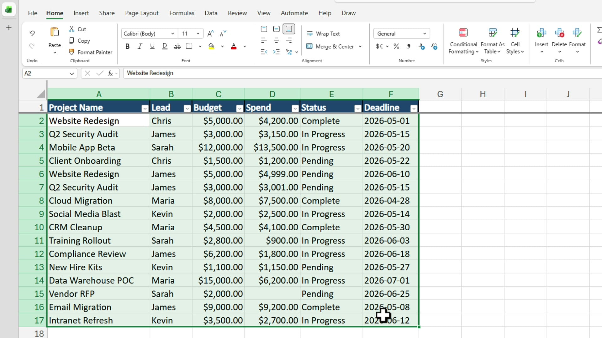
Click cell A2 and drag down to F17 — every row you want the rule to evaluate, excluding the header row in row 1. The active cell stays at A2 and the rest of the range fills with the green selection color.

Excel data range A2:F17 selected before applying conditional formatting — Select the entire data range from A2 to F17 — every row you want the rule to evaluate. Skip the header row.

Step 2: Open Conditional Formatting and pick New Rule

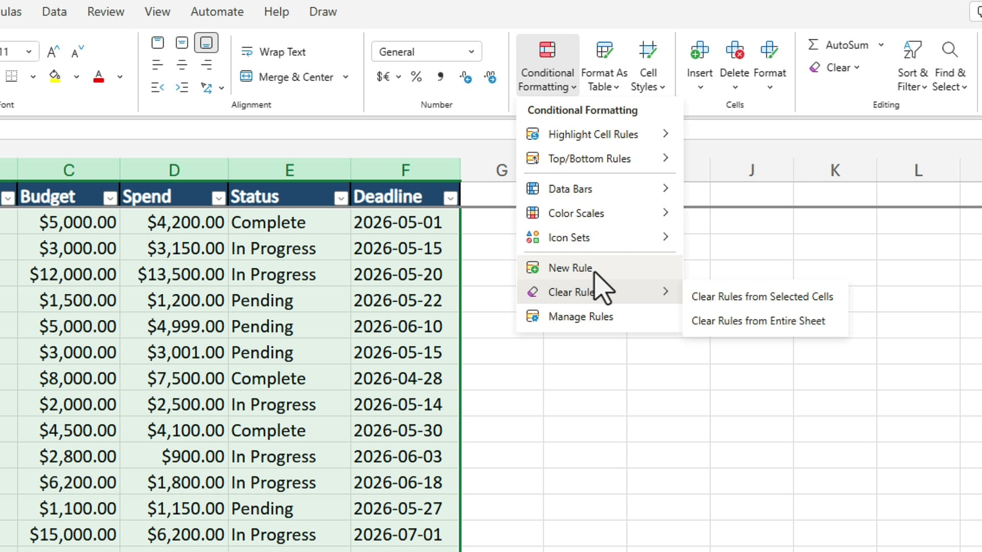
With the range still selected, go to the Home tab and click Conditional Formatting. From the dropdown, choose New Rule.

Conditional Formatting menu open on the Home tab in Excel for the web with New Rule option visible — On the Home tab, open the Conditional Formatting dropdown and choose New Rule. The location is identical in Excel desktop.

In Excel for the web, the rule builder slides out as a task pane on the right. In Excel desktop you get the same dialog as a popup. Both behave identically from here.

Step 3: Write the formula =$D2>$C2

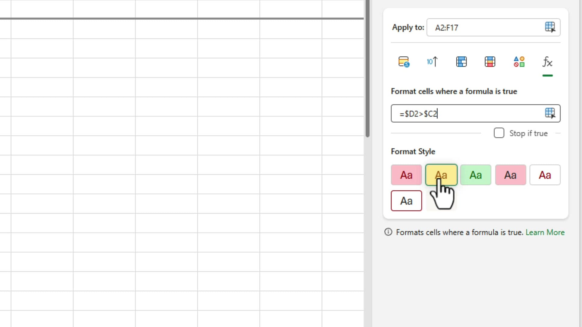
At the top of the task pane, click the fx icon to switch to a formula-based rule. The Apply to box should already show A2:F17. In the formula box, type:

=$D2>$C2

That is the entire rule. It reads: "for every cell in the selected range, compare the value in column D of that row to the value in column C of that row, and if D is greater, format the cell."

Why the dollar signs matter

Putting $ in front of the column letter (but not the row number) creates a mixed reference. The column is locked — Excel always looks at column D and column C — but the row is free, so the rule walks down row by row: row 2 compares D2 to C2, row 3 compares D3 to C3, and so on. Without the dollar signs the rule would drift sideways and highlight the wrong cells.

If mixed references still feel fuzzy, this is the moment to read my deeper walkthrough on mixed and absolute references in conditional formatting — it is the single concept that unlocks 90% of formula-based rules.

Excel conditional formatting rule with formula equals dollar D2 greater than dollar C2 and yellow format style selected — Choose the fx (formula) option, type =$D2>$C2, and pick the yellow Format Style. The Apply to box shows A2:F17 — the range you selected.

Step 4: Pick a color and click Done

Under Format Style, click the yellow swatch (or any color you prefer). Click Done and close the task pane.

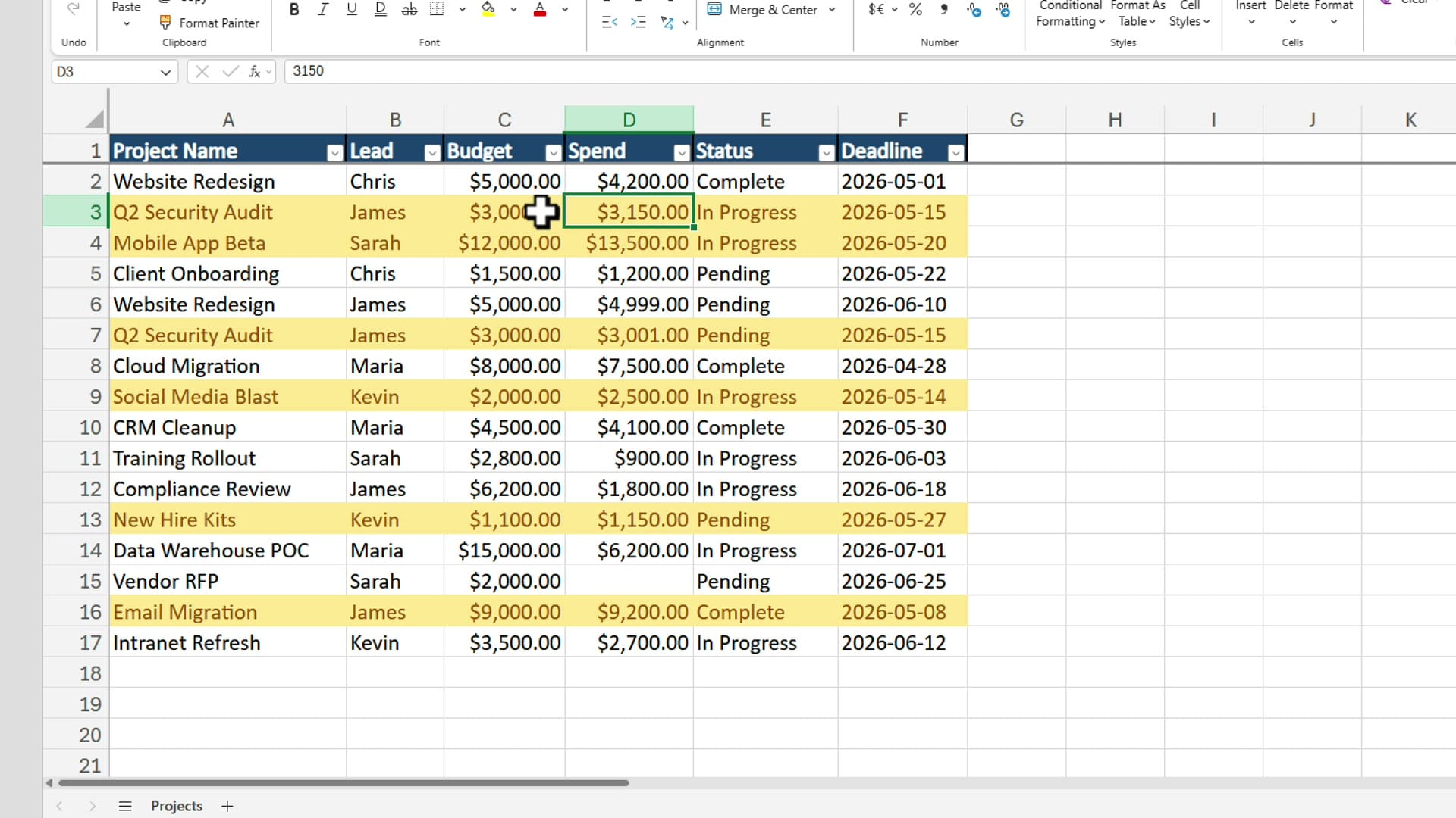
Excel rows highlighted yellow where the spend amount exceeds the budgeted amount — Every row where Spend exceeds Budget now lights up yellow. Rows 3, 4, 7, 9, 13, and 16 are over budget.

Every row where Spend exceeds Budget is now highlighted. Row 3 — Q2 Security Audit — went $150 over its $3,000 budget, so the whole row turns yellow. Row 9, Social Media Blast, went $500 over, also yellow.

Step 5: Test the rule live

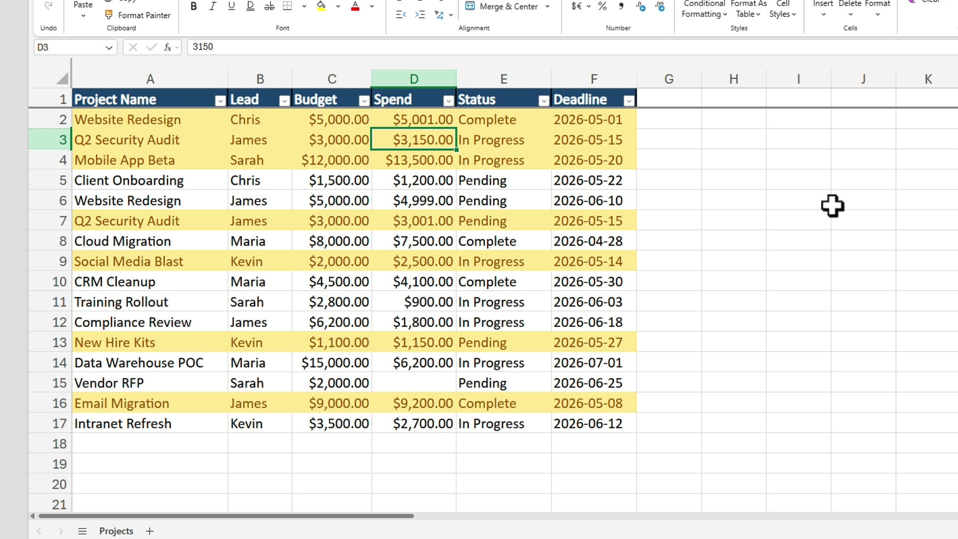
Conditional formatting is dynamic — change a number and the formatting updates instantly. Change D2 to 5,001 and watch row 2 turn yellow (it is now $1 over budget).

Row 2 in Excel highlighted yellow after changing the spend amount to be larger than the budget — Test it: change D2 to 5,001 (just $1 over budget) and row 2 immediately turns yellow. Change a spend back below budget and the yellow disappears.

Then change D3 to 2,950 and the yellow on row 3 disappears, because spend is no longer over the budget. This is what makes the rule useful in a living report — you do not have to re-apply it after edits.

An easier alternative: add a Difference column

The way the question came in had no helper column. If you control the spreadsheet, I usually suggest adding one — it makes the report more readable and the conditional formatting rule simpler.

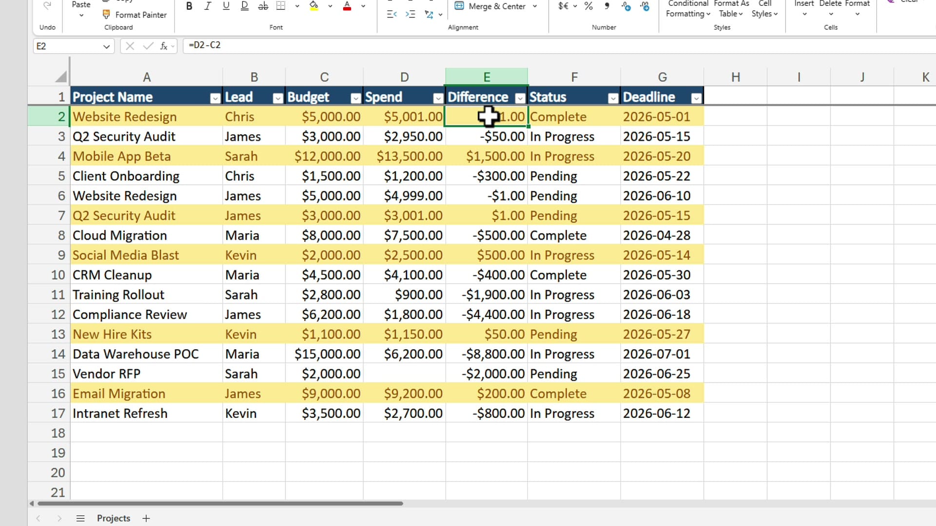
Excel helper column with formula equals D2 minus C2 showing positive and negative differences — Alternative approach: add a Difference column with =D2-C2 and base the rule on that single column being greater than 0. Useful when you want the number itself in the report.

Add a Difference column (column E here) with =D2-C2. Positive numbers are over budget, negative numbers are under. Now your conditional formatting rule can simply test that one column — =$E2>0 — instead of comparing two columns. Same yellow result, but the number itself becomes a useful KPI you can sort, filter, or chart.

Either approach works. Pick whichever fits the way the rest of your report is structured.

Where to go next

If you are new to conditional formatting, start with the getting started guide with five examples — it covers the basic rule types before you ever touch a formula. If you need to combine two tests in one rule (for example, over budget and still In Progress), see conditional formatting with the AND function.

The formula technique you just learned is the building block for everything else: highlighting every nth row, flagging duplicates across rows, or shading anything based on a date in another column all work the same way — select the range, write one formula with the right dollar signs, pick a color.