Microsoft Excel

Find and Remove Duplicates in Excel: 3 Methods with UNIQUE, VSTACK, and TEXTJOIN

Finding duplicates, highlighting them, and removing them is something I do all the time in Excel. There's no single best tool for the job — the right approach depends on whether your data has a unique identifier, whether you need to compare one list or two, and whether you want to count results or just clean things up.

In this guide I'll walk through three examples that cover the situations you'll run into most often.

The sample file is available for download below.

excel duplicates three examples with unique

excel duplicates three examples with unique.xlsx

12 KB

Three Excel lists used in the duplicates tutorial — The three datasets we'll work with: List 1 (simple list with duplicates), List 2 (names with cities and no unique identifier), and List 3A/3B (two lists to compare).

Example 1: Highlight, Count, and Remove Duplicates in a Single List

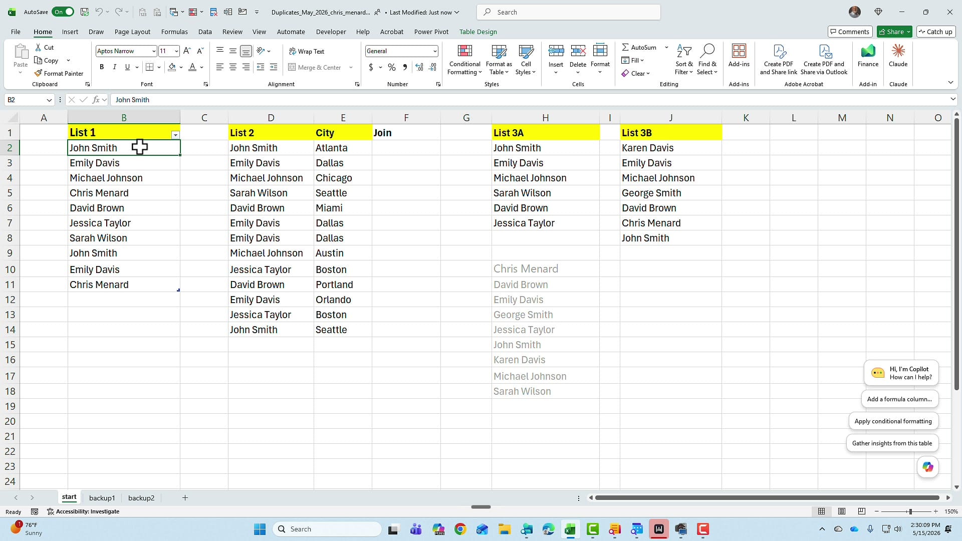
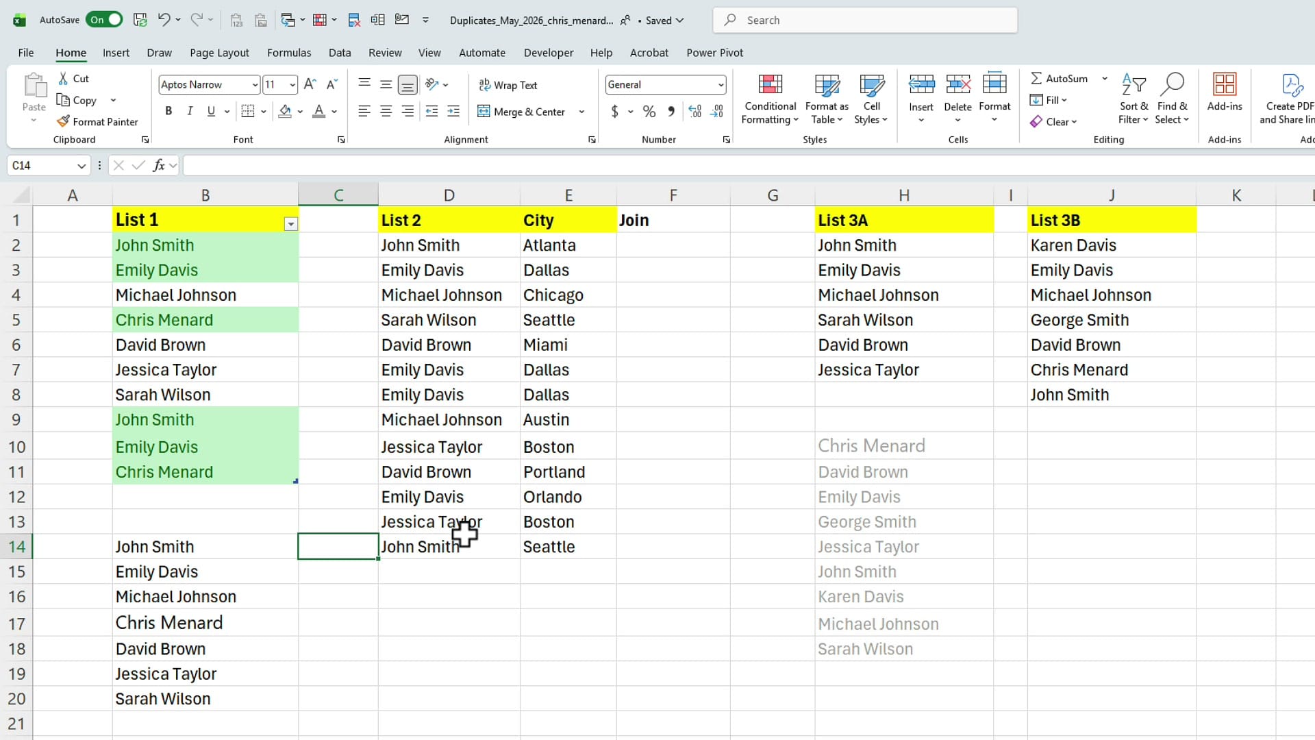
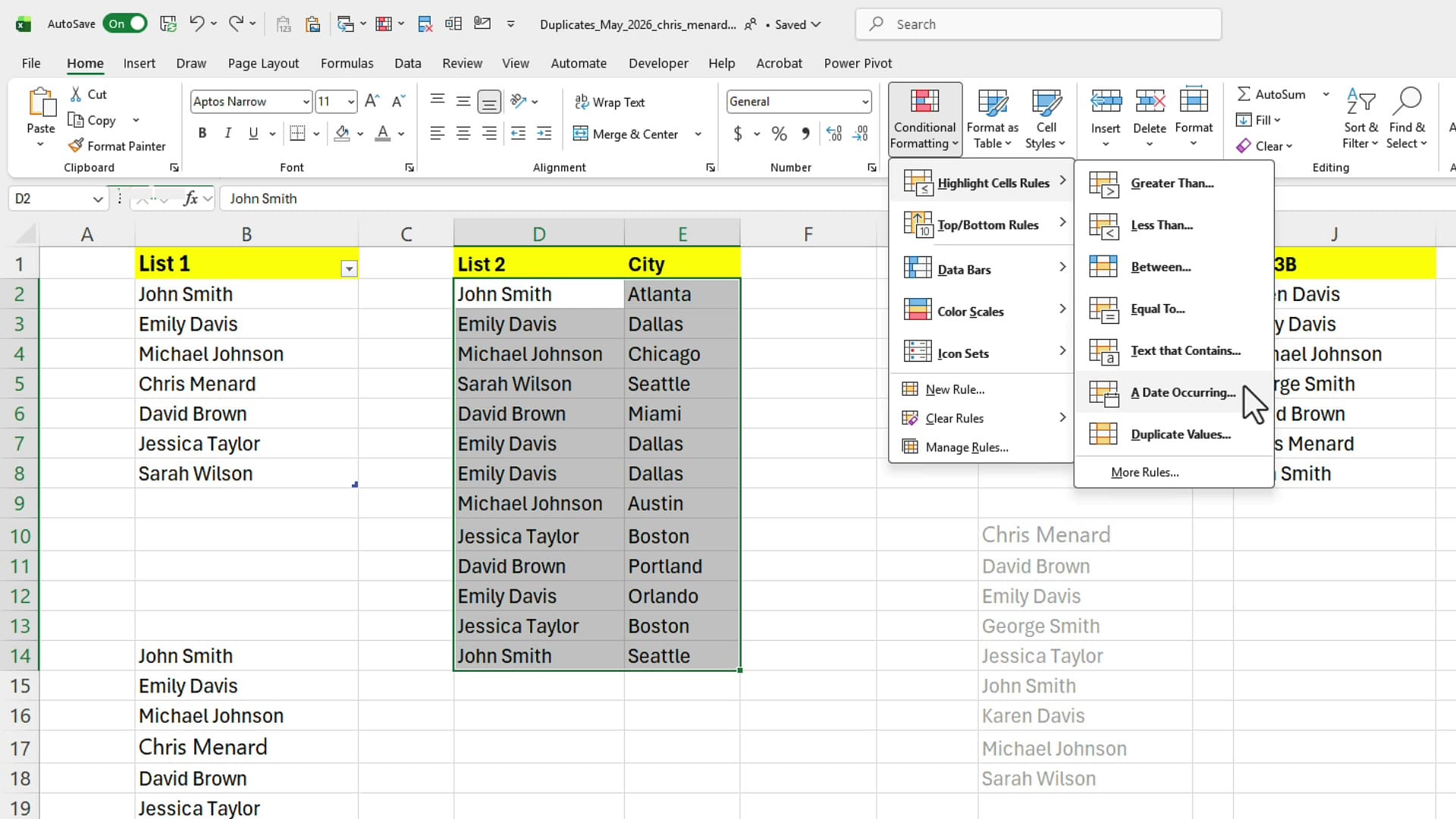
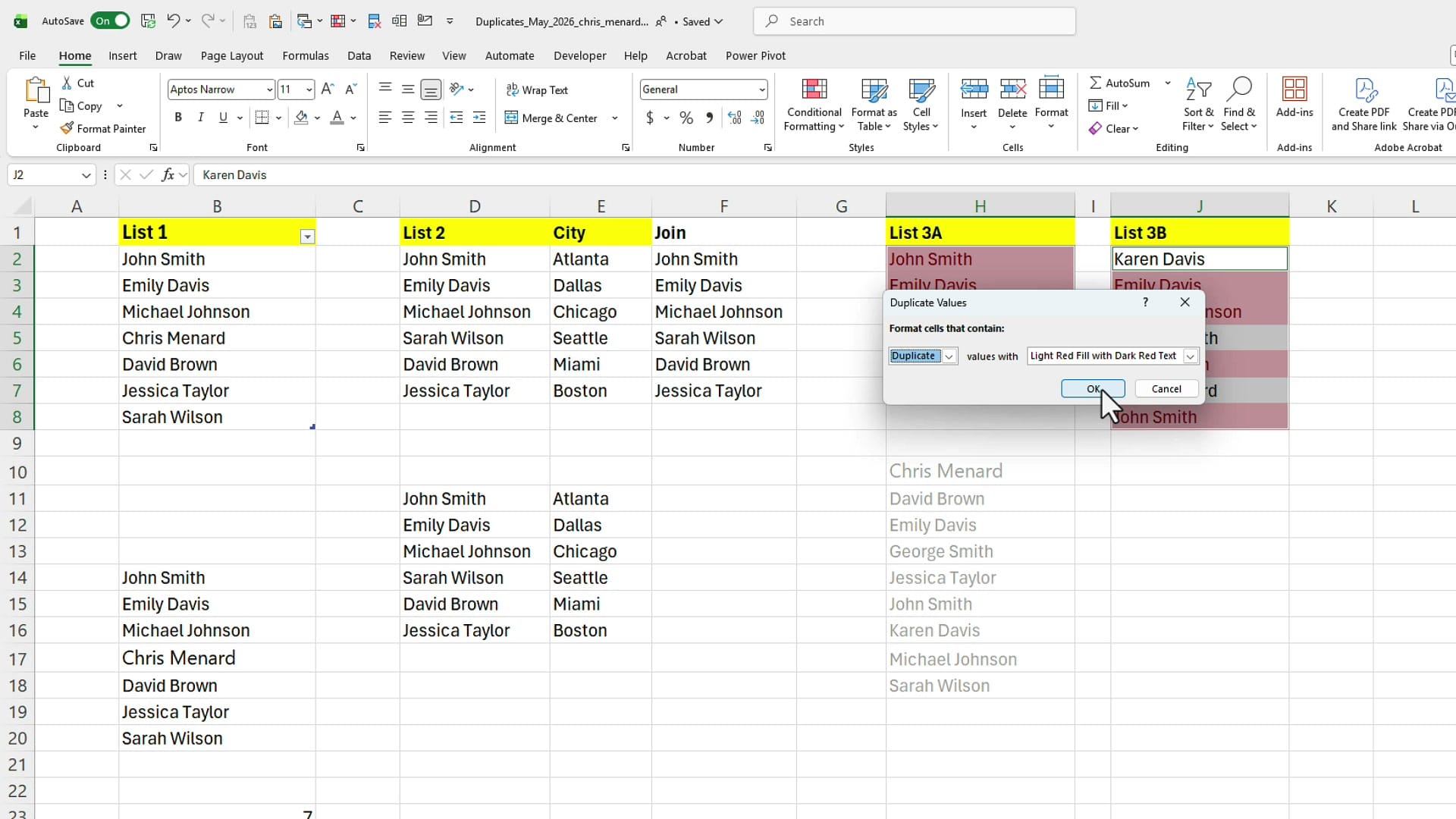
For the first example, look at List 1. Before you remove anything, it's a good idea to see what you're dealing with. Highlight the list, then on the Home tab go to Conditional Formatting → Highlight Cells Rules → Duplicate Values. You can change the fill colour if you don't like the default; once you click OK, every duplicate is shaded.

List 1 duplicates highlighted with green conditional formatting — Conditional formatting reveals which names in List 1 appear more than once. This is always my first step — visual confirmation before any data is removed.

Pull a clean list with UNIQUE

Before removing anything, you can use the UNIQUE function to spill the distinct values out into another column. The formula is simply =UNIQUE(Table1[List 1]) — or you can point it at a plain range instead of a table. Excel spills the unique names automatically.

Counting unique values — the right way

There's a quick-and-dirty way to count uniques: highlight the UNIQUE spill range and read the count off the status bar at the bottom right of Excel. Type that number into a cell, paste it, done. It works, but it's a workaround. If anything in the source data changes, that hard-coded number will be wrong.

The better method is to wrap UNIQUE inside COUNTA: =COUNTA(UNIQUE(Table1[List 1])). This is a dynamic formula — if you add a new name or remove one upstream, the count updates instantly. It's a small change with a big payoff in spreadsheets that get edited regularly.

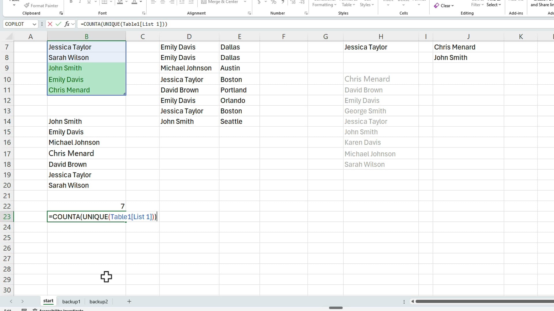
COUNTA UNIQUE formula counting distinct names in List 1 — `=COUNTA(UNIQUE(Table1[List 1]))` returns a live count of distinct values. Unlike the static method, this updates whenever the source data changes.

Actually removing duplicates with the Data tab

UNIQUE shows you what the clean list looks like, but it doesn't change the original data. To delete the duplicates in place, click anywhere inside the data, switch to the Data tab, and click Remove Duplicates — one of my favourite features in Excel.

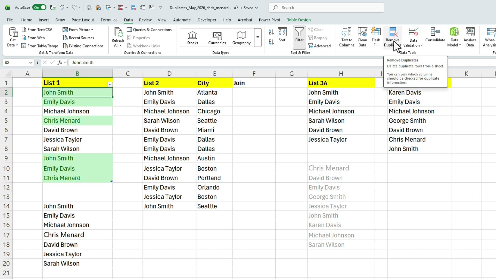
Remove Duplicates button on the Data tab with tooltip — The Remove Duplicates tool on the Data tab. Excel automatically detects the header row and shows which column it's checking.

Excel detects the header row, asks you which column to check (in this case, List 1), and reports back: 7 unique values remain. That matches what UNIQUE showed, so the numbers line up.

Example 2: Removing Duplicates When There's No Unique Identifier

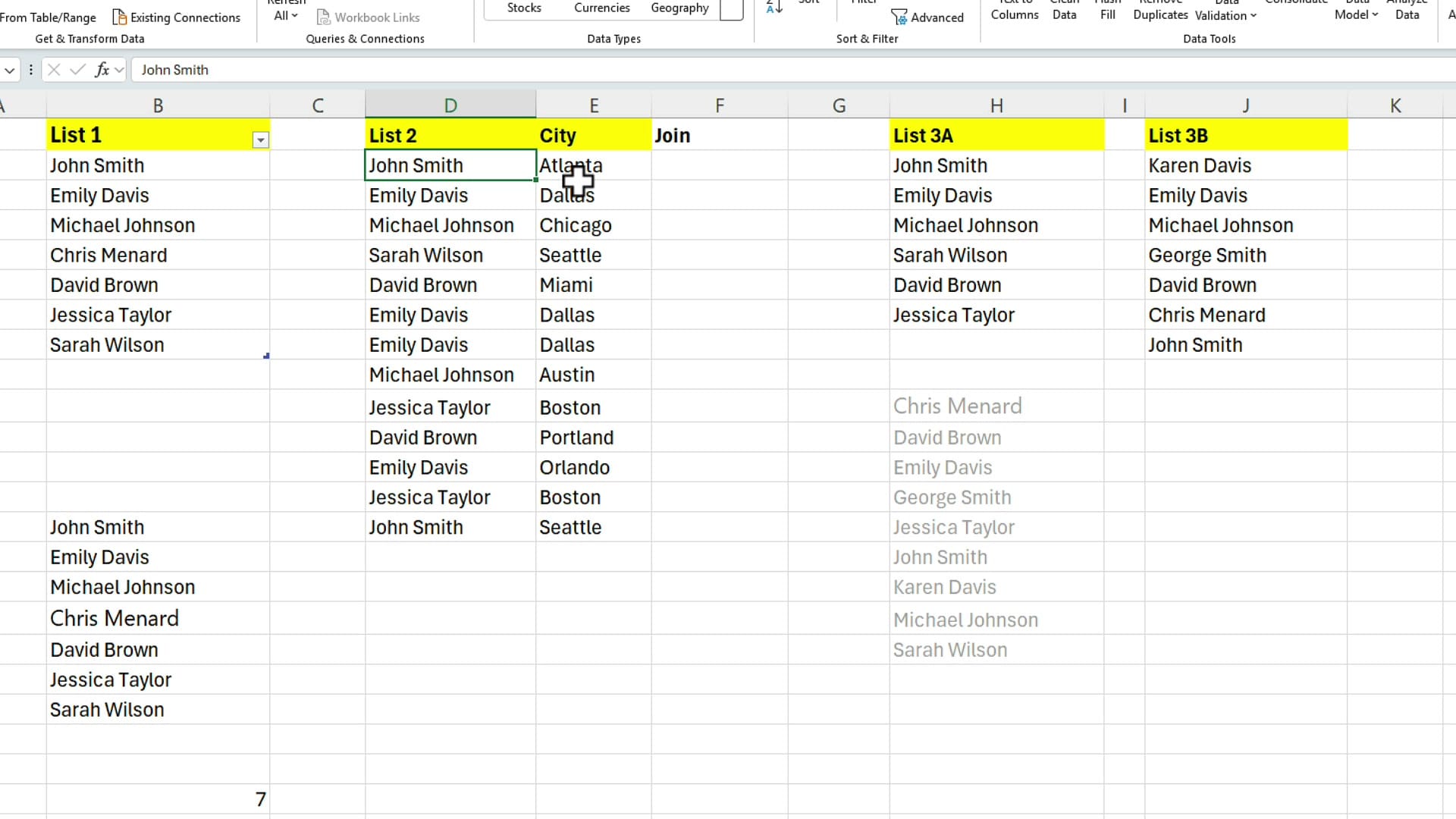
List 2 is where things get interesting. We've got names paired with cities — for instance, John Smith in Atlanta and John Smith in Seattle. Both rows are valid records of different people. There's no employee ID, customer number, or order number to tell them apart. That's a problem, because it means the same name can legitimately appear more than once.

Excel list of names and cities with no unique identifier column — List 2 has names paired with cities but no unique identifier. John Smith appears twice — once in Atlanta, once in Seattle — and these are different people.

Two common mistakes to avoid

If you click into this data and run Remove Duplicates against just the name column, Excel will quietly delete the second John Smith. Sometimes that's correct; often it isn't. You don't want a tool making that judgement for you.

The second mistake is highlighting either column on its own and applying Duplicate Values conditional formatting. Run it on the City column and Seattle gets flagged as a duplicate — even though it's the city for two completely different records. Conditional formatting on a single column isn't comparing the whole row, so it flags things that aren't actually duplicates.

Excel Home tab Conditional Formatting menu showing Highlight Cells Rules and Duplicate Values — The Conditional Formatting menu. Highlight Cells Rules → Duplicate Values only compares within the selection — it won't catch row-level duplicates across multiple columns.

The fix: a helper column with TEXTJOIN

The workaround I use all the time is to build my own unique identifier by combining the name and city into a single helper column. You can use CONCATENATE, but TEXTJOIN is cleaner: =TEXTJOIN(", ", TRUE, D2, E2). The first argument is the delimiter, the second tells Excel to ignore empty cells, then you list the columns to join.

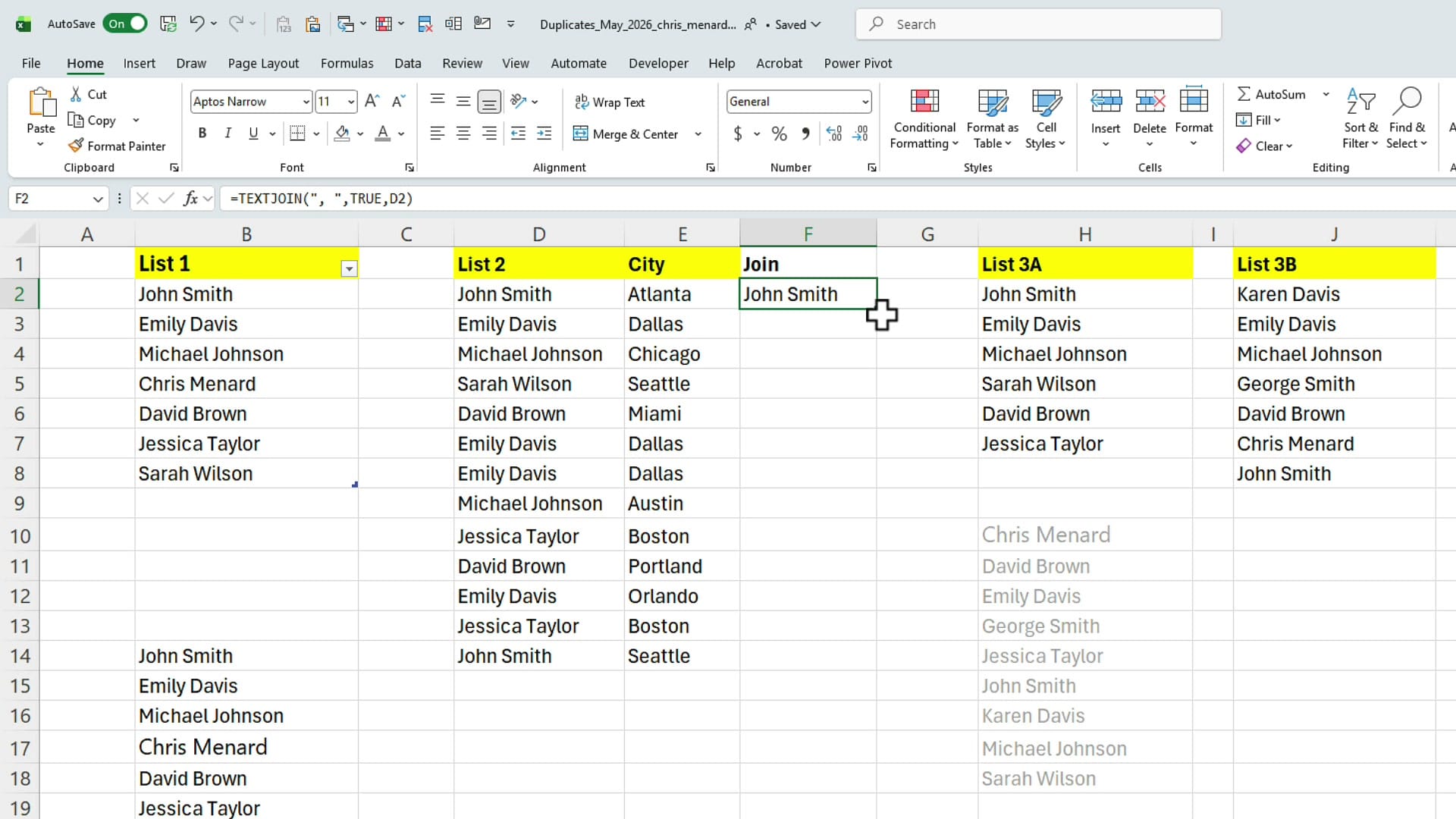
Excel TEXTJOIN formula creating a helper column combining name and city — The TEXTJOIN helper column gives each row a true unique identifier — "John Smith, Atlanta" and "John Smith, Seattle" are now distinct.

Pull that down through the whole list and you've got a Join column where each row has a real unique identifier — "John Smith, Atlanta" is now different from "John Smith, Seattle".

Remove Duplicates against the helper column only

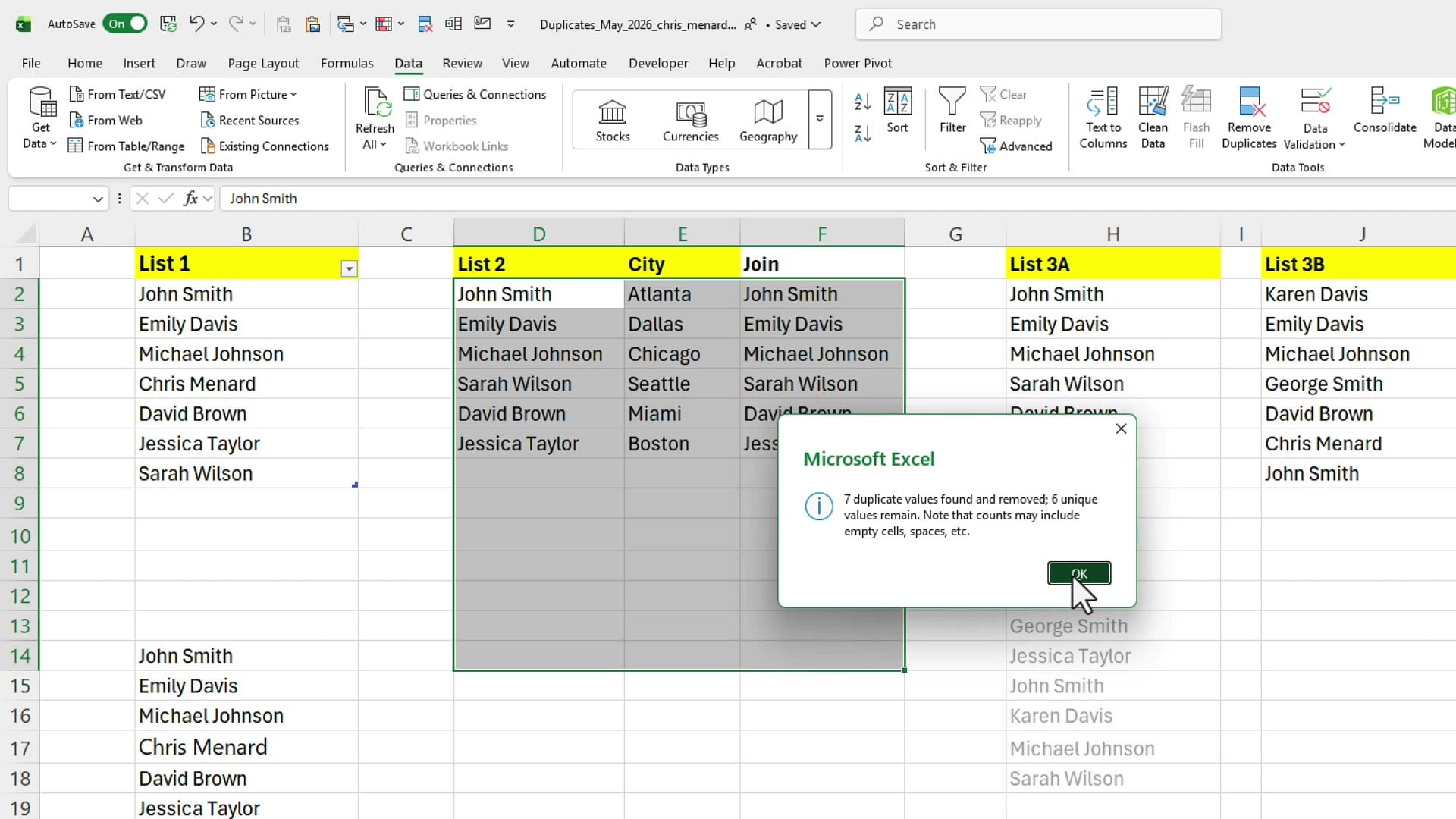
Now highlight everything and go back to Data → Remove Duplicates. This time, uncheck List 2 and City — you only want Excel to check the Join column. Click OK and Excel correctly identifies and removes the row-level duplicates.

Excel dialog showing 7 duplicate values found and removed, 6 unique values remain — Excel confirms 7 duplicates were found and 6 unique values remain. The Join column was the key — checking the name or city alone would have given the wrong result.

If you'd like a running count of unique values, the same =COUNTA(UNIQUE(...)) pattern from Example 1 works just as well here.

Example 3: Finding Duplicates Across Two Separate Lists

The third scenario is comparing two lists side by side — List 3A and List 3B — to find names that appear in both. The simplest visual approach: highlight the first list, hold down the Ctrl key, highlight the second list, then run Conditional Formatting → Highlight Cells Rules → Duplicate Values. Anything appearing in both lists is now shaded.

Excel Duplicate Values dialog highlighting names appearing in both List 3A and List 3B — Holding Ctrl while selecting both columns, then applying Duplicate Values conditional formatting, instantly shows which names appear in both lists. Change a name to something unique and you'll see the highlight drop in real time.

Count distinct names across both lists with VSTACK, UNIQUE, and SORT

To get a single list of every distinct name across both columns — deduplicated and sorted — combine three functions: VSTACK stacks the ranges vertically, UNIQUE strips duplicates, and SORT orders the result. The formula is:

=SORT(UNIQUE(VSTACK(H2:H7, J2:J8)))

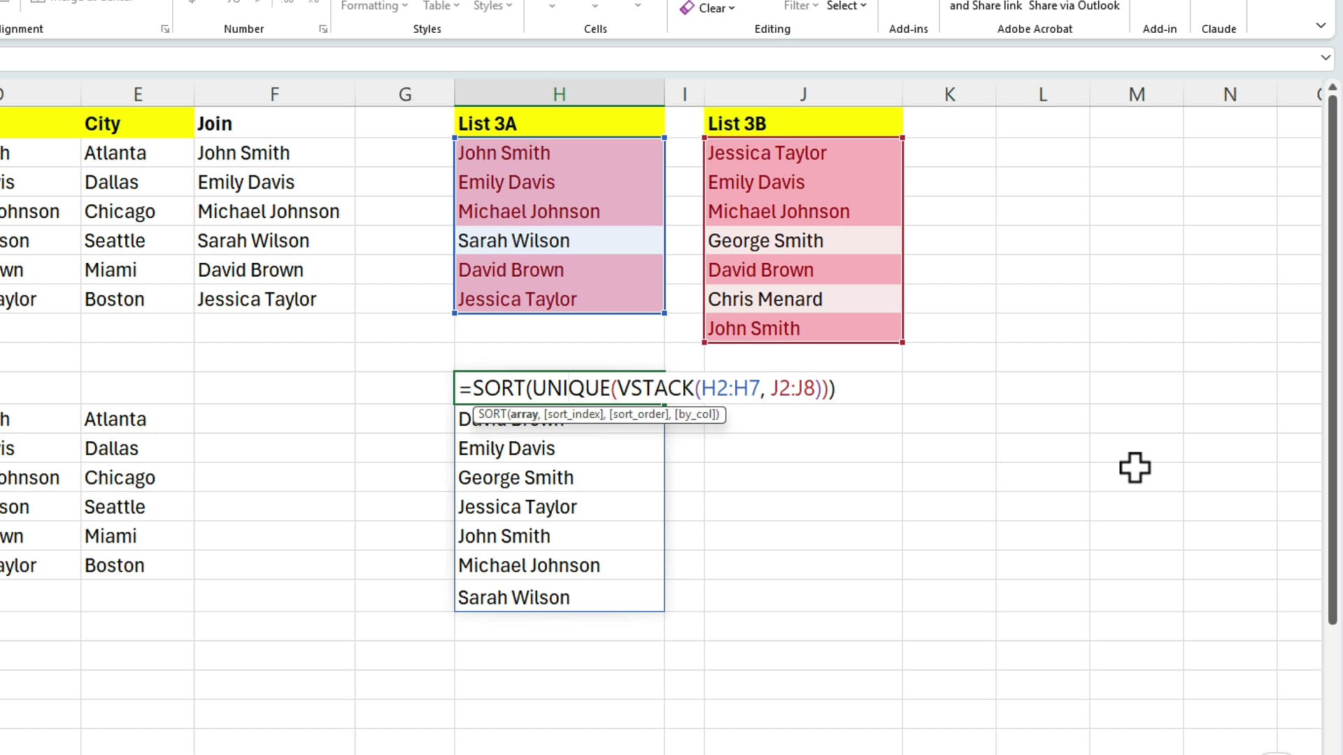
Excel SORT UNIQUE VSTACK formula stacking two lists into a single sorted unique list — VSTACK pulls List 3A and List 3B into one range, UNIQUE removes duplicates, and SORT orders the result alphabetically — all in a single formula.

VSTACK is the function that makes this possible — before it existed, combining two non-contiguous ranges into one was a much bigger job. Now it's a single inner function call.

Counting the distinct names across both lists

To get the total count of distinct names across both lists in a single cell, wrap the whole thing in COUNTA: =COUNTA(UNIQUE(VSTACK(H2:H7, J2:J8))). Same pattern as Example 1, just with VSTACK adding the second range into the mix.

Quick reference

Situation	Best tool
Simple single-column list	Conditional Formatting → Duplicate Values, then Remove Duplicates
Count distinct values dynamically	`=COUNTA(UNIQUE(range))`
Multi-column data, no unique ID	TEXTJOIN helper column, then Remove Duplicates on the helper
Compare two separate lists	Ctrl-select both ranges, then Duplicate Values conditional formatting
Stack two lists into one sorted unique list	`=SORT(UNIQUE(VSTACK(range1, range2)))`

That's three different scenarios — one list, multi-column without an identifier, and two separate lists — all handled with the same handful of tools: Conditional Formatting, Remove Duplicates, UNIQUE, COUNTA, TEXTJOIN, VSTACK, and SORT. For the next level of duplicate handling I'd reach for Power Query, which is worth a separate post on its own.

I hope this was a useful introduction to handling duplicate values in Excel. Thanks for reading and have a wonderful day.

UNIQUE Function in Excel - Dynamic Array Formula

Excel’s UNIQUE function will return a unique list from a range. The results will automatically "spill" into an adjacent range of the appropriate size.