Microsoft Excel

Excel's New List Feature: Filter and Count Multiple Items in One Cell

Excel can now hold a list of items in one cell. Create lists with Ctrl+J, filter by a single name, and summarize them with FLATTEN, UNIQUE, SORT, and COUNTIF.

Microsoft Excel has a great new feature rolling out: the ability to hold multiple items inside of one cell. If you have ever typed several names into a single cell separated by commas, you already know the problem. Excel treats the whole thing as one piece of text, so you cannot filter on just one of those names or easily count how often each one appears. A list fixes both.

Excel New List Feature

Download the practice file and test this yourself.

Excel_new_list_feature.xlsx

19 KB

Below I create a list in a cell, convert existing comma-separated names into lists, filter by a single name, and then summarize everything with the new FLATTEN function combined with UNIQUE, SORT, and COUNTIF.

Check that you are on the Beta Channel

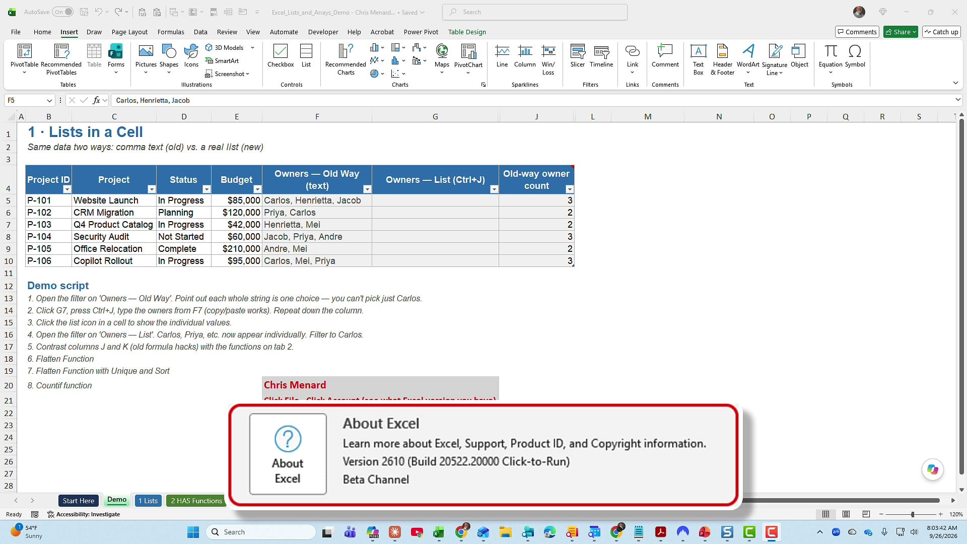
Right now, lists are only available to Beta Channel users. To see which channel you are on, open Excel, go to File, and click Account. The channel is listed under About Excel. Mine shows Version 2610 (Build 20522.20000), Beta Channel.

About Excel panel showing Version 2610, Build 20522.20000, Beta Channel, over a worksheet titled Lists in a Cell — File > Account shows your version and channel. Lists in cells are currently rolling out to the Beta Channel.

The problem with comma-separated names

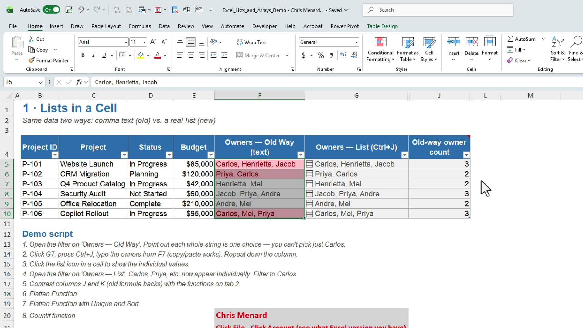
My example is a small project table. Column F holds the project owners, and most projects have more than one, so the names are typed into a single cell with commas between them: Carlos, Henrietta, Jacob.

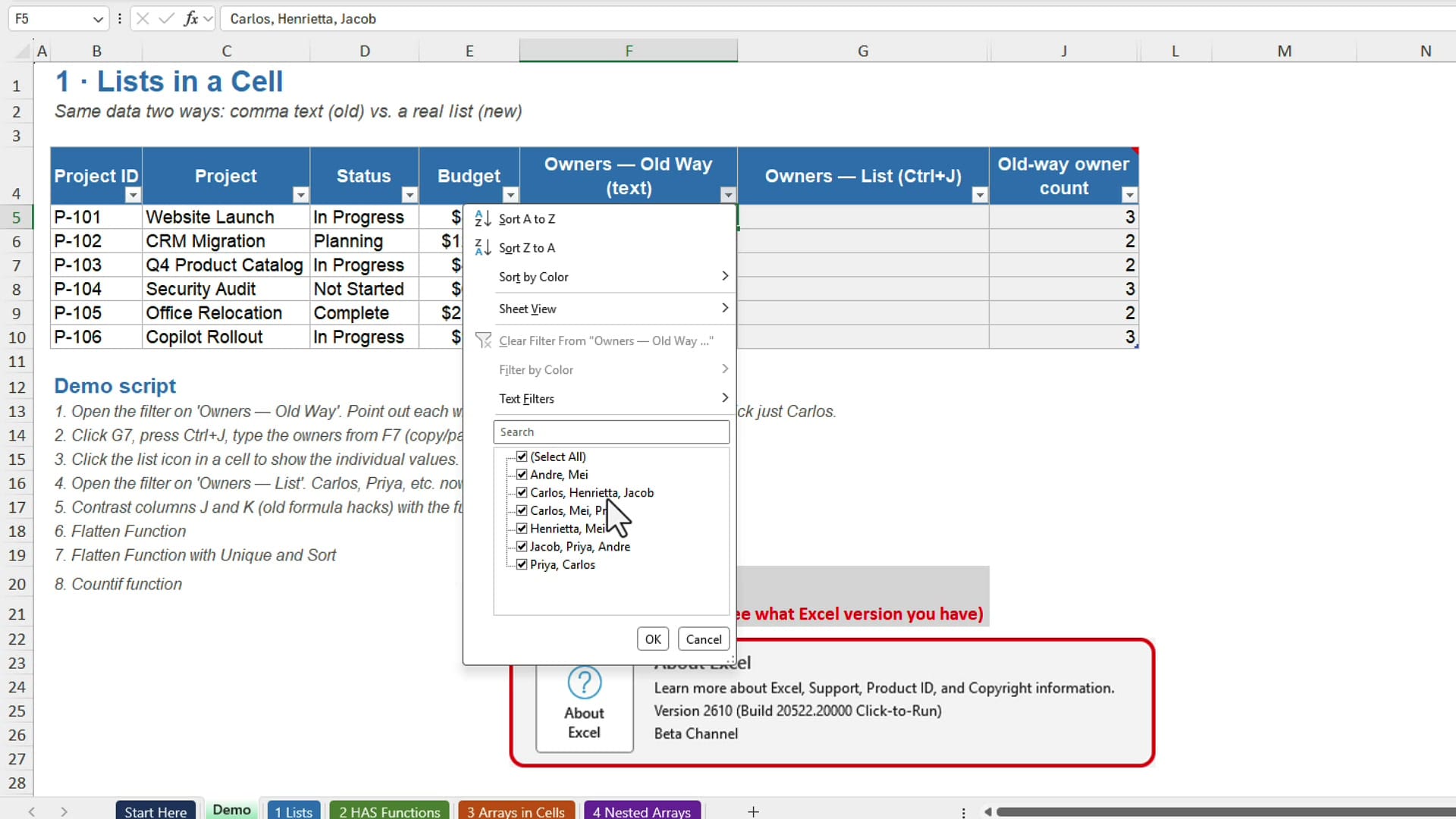
Click the filter dropdown on that column and try to find just Carlos. You can't. Every choice in the filter is the entire string, so Carlos shows up bundled with other names in three different entries. Yes, I could go to Text Filters and use Contains, but that is a lot of work for something this basic.

Excel filter dropdown on a comma-separated Owners column listing whole strings such as Carlos, Henrietta, Jacob and Priya, Carlos as single choices — With comma-separated text, each full string is one filter choice. There is no way to check just Carlos.

Create a list in a cell

The new feature is called List. If you are a mouse person, go to the Insert tab and click List in the Controls group, right next to Checkbox.

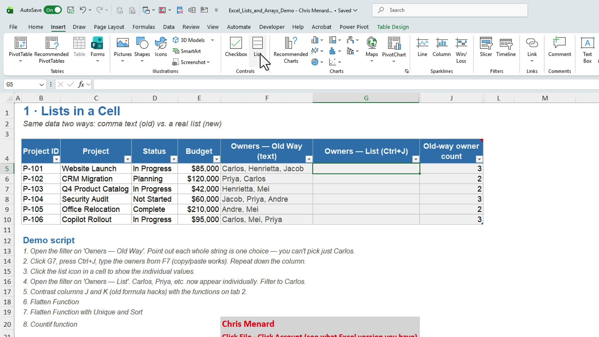
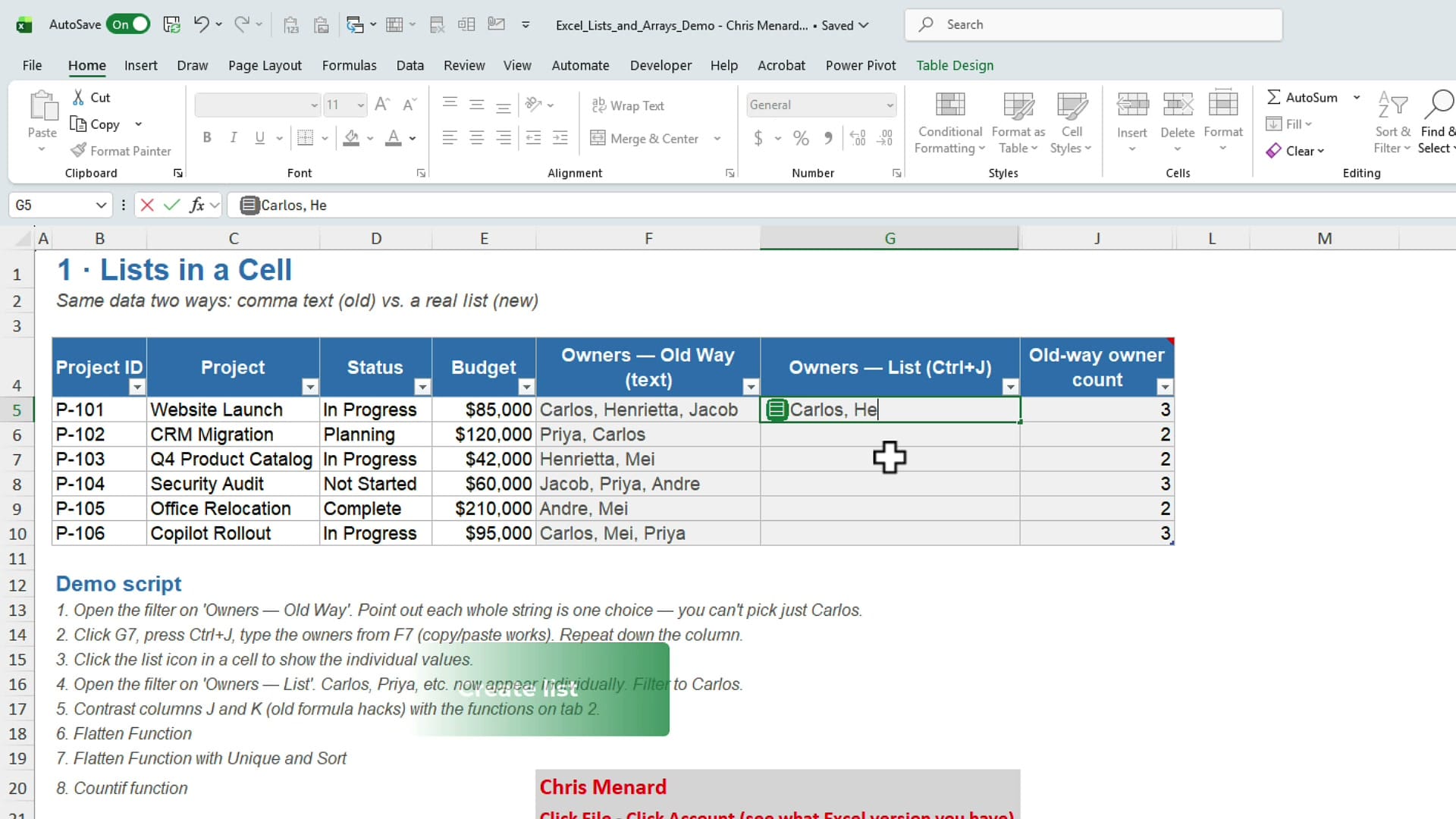
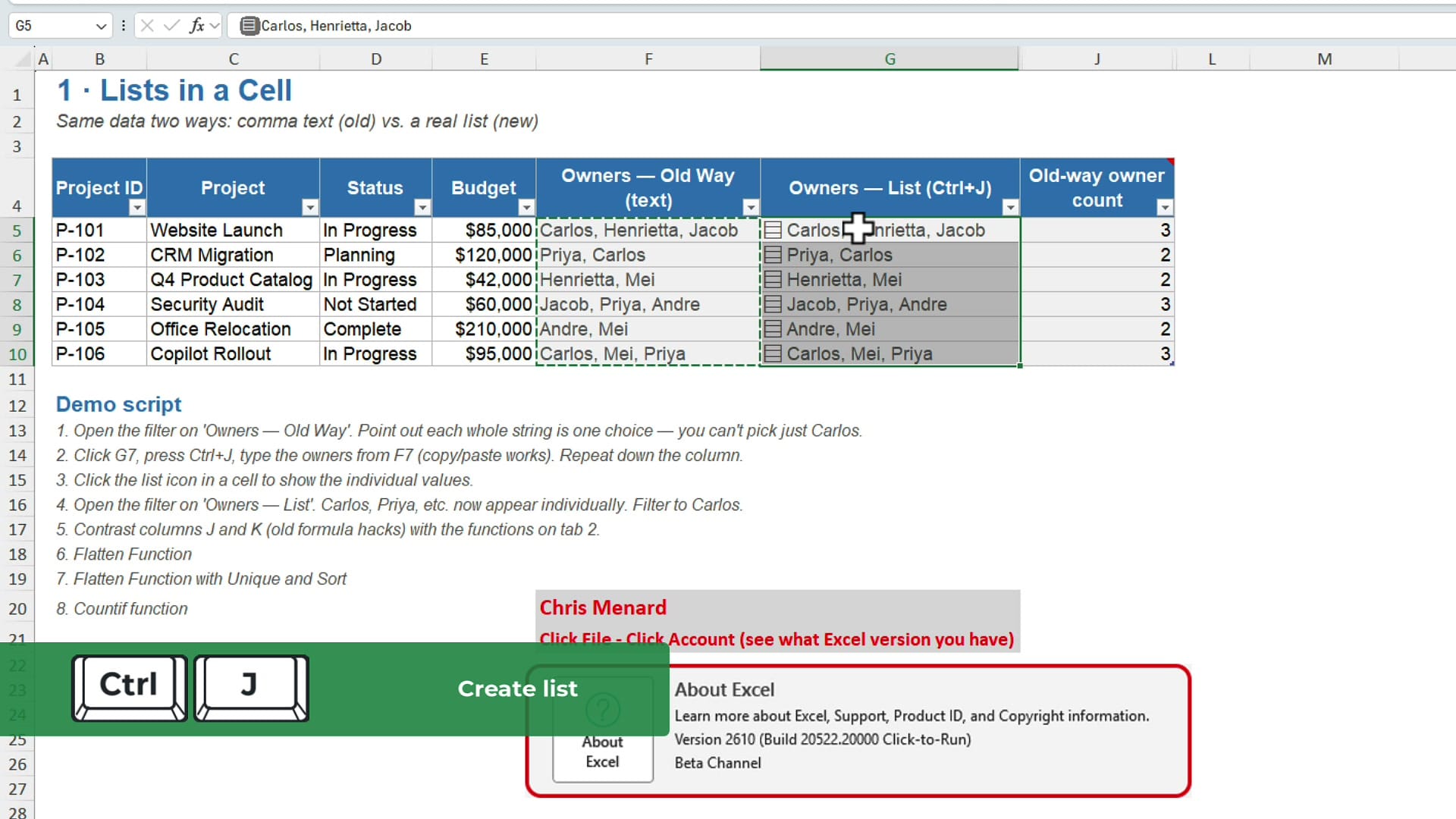
Excel Insert tab with the List button in the Controls group next to Checkbox, and an empty cell G5 selected — Insert > List turns the selected cell into a list.

I am going to stick with the keyboard: Ctrl + J. A small list icon appears at the left edge of the cell. Type the names with commas between them, then press Enter.

Excel cell G5 showing a green list icon while names are typed in, with a Ctrl J Create list keyboard callout — Ctrl + J creates the list. The icon in the cell and in the formula bar tells you this is a list, not plain text.

Now open the filter dropdown on that column. Carlos is by himself, and so are Henrietta and Jacob. Each item in the list is its own filter choice. Excel also shows a Blanks entry at this point, because the other cells in the column are still empty.

Convert existing names into lists

That first cell is the only list of names I am going to type. You do not have to retype data you already have. I could select the names in column F and press Ctrl + J right there, but I want to keep the original column for comparison, so I copy the old names, paste them into the list column, and with the pasted cells still selected, press Ctrl + J.

Excel column G with six cells converted to lists, each showing a list icon, next to the original comma-separated text in column F — Paste the comma-separated text, keep the cells selected, and press Ctrl + J. Every cell becomes a list in one step.

Filter by a single list item

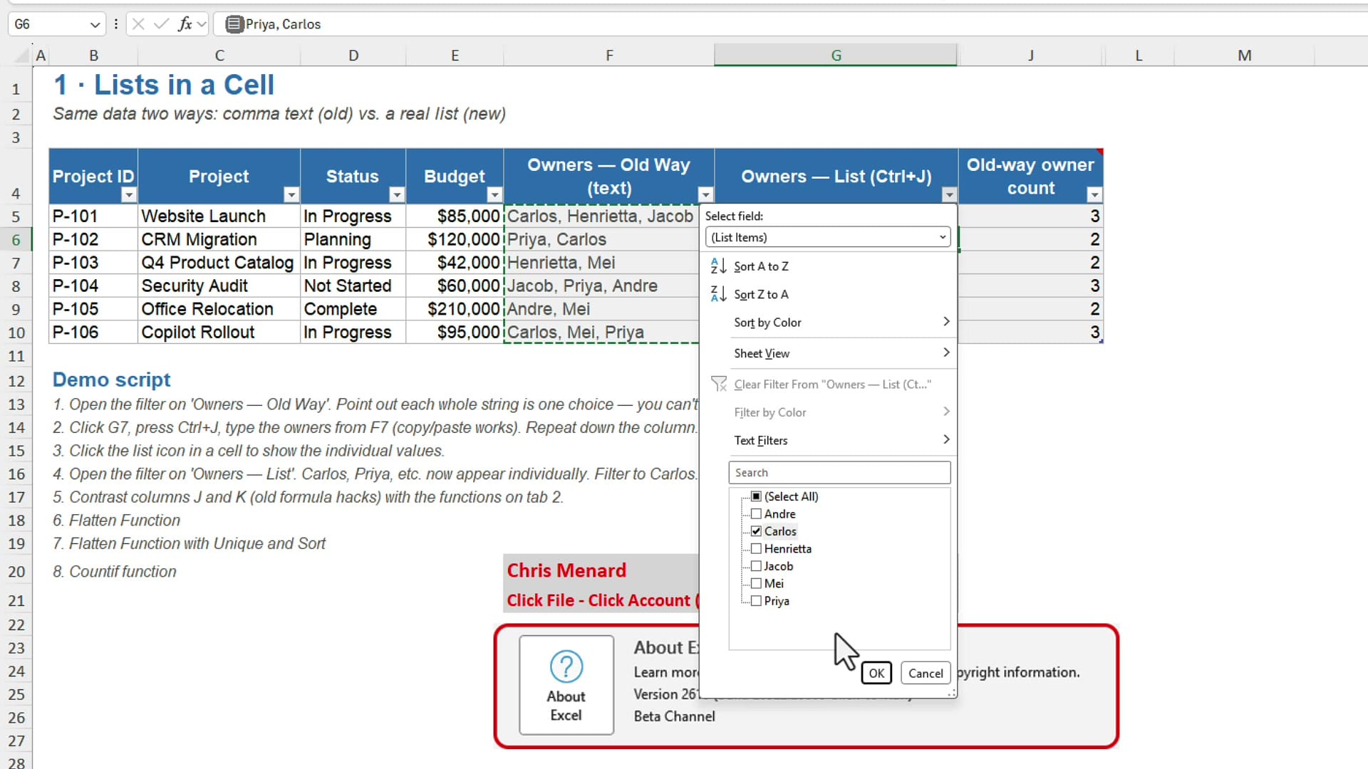
Click the filter dropdown again. All of the names are there, one per line: Andre, Carlos, Henrietta, Jacob, Mei, Priya. There are no blanks now, and the names are in alphabetical order. Check Carlos, click OK, and the table shows only the three projects Carlos is on.

Excel filter dropdown on the list column showing individual names Andre, Carlos, Henrietta, Jacob, Mei, and Priya with only Carlos checked — With a list column, every name is its own checkbox. Filtering for Carlos takes one click.

Switch between list items and display values

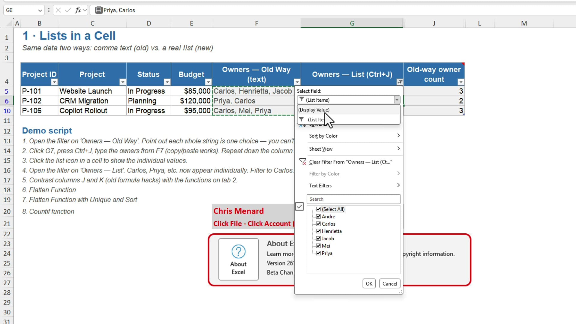
Look at the top of the filter menu for a list column. There is a new Select field dropdown with two choices: List Items and Display Value. List Items filters on the individual names. Display Value filters on the whole cell the way a normal text column would, so you see Carlos, Henrietta, Jacob as a single choice again. You can toggle back and forth between the two. I keep mine on List Items.

Excel filter menu for a list column with the Select field dropdown open showing Display Value and List Items options — The Select field dropdown at the top of the filter menu switches between individual list items and the full display value.

Counting owners the old way

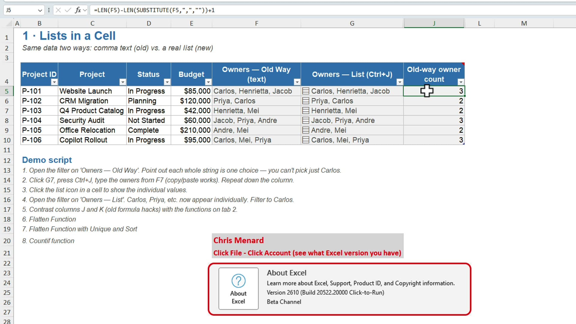
Lists also make counting much easier. Here is what I had before. The last column of my table counts the owners in each cell of the old text column with this formula:

=LEN(F5)-LEN(SUBSTITUTE(F5,",",""))+1

It measures the length of the text, measures it again with the commas removed, and adds one. That is a pretty detailed formula for a simple question, and all it gives me is the number of names in each cell.

Excel formula bar showing a LEN and SUBSTITUTE formula that counts the owners in a comma-separated cell, returning 3 — The old approach: count the commas and add one. It works, but only cell by cell.

It does not tell me how many projects Carlos is on. To check that, I select the old owners column and add a quick conditional formatting rule: Home > Conditional Formatting > Highlight Cells Rules > Text that Contains, and type Carlos. Three cells light up. Change the rule to Jacob and two cells light up. When I am done, I clear it with Conditional Formatting > Clear Rules > Clear Rules from This Table.

Excel old owners column with three cells highlighted in red by a conditional formatting rule for text containing Carlos — A Text that Contains rule confirms Carlos appears in three cells. Keep those numbers in mind for the next step.

Expand the lists with FLATTEN

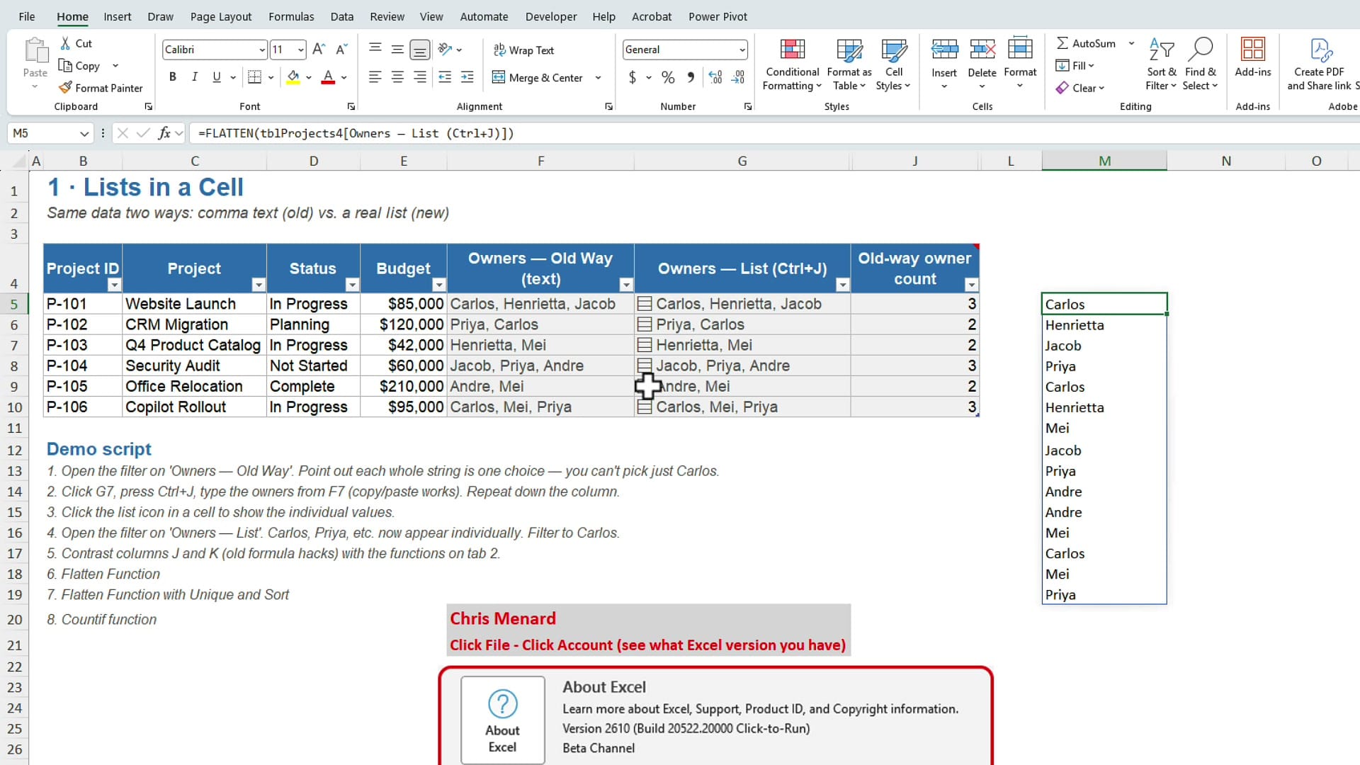
Now the new way. Alongside lists, Excel has a new function called FLATTEN. Point it at the list column and it spills every item from every list into a single column:

=FLATTEN(tblProjects4[Owners — List (Ctrl+J)])

My data is in a table, so clicking the column gives me a structured reference with the table name instead of a cell range. The result is one long column with one name per row.

Excel FLATTEN formula in cell M5 spilling fifteen individual owner names down column M from the list column — FLATTEN takes the six list cells and returns all fifteen names in one spilled column.

Remove duplicates and sort the names

FLATTEN keeps repeating names, because Carlos is in there more than once and so is Jacob. Wrap the formula in UNIQUE to remove the duplicates, then wrap that in SORT to put the names in order:

=SORT(UNIQUE(FLATTEN(tblProjects4[Owners — List (Ctrl+J)])))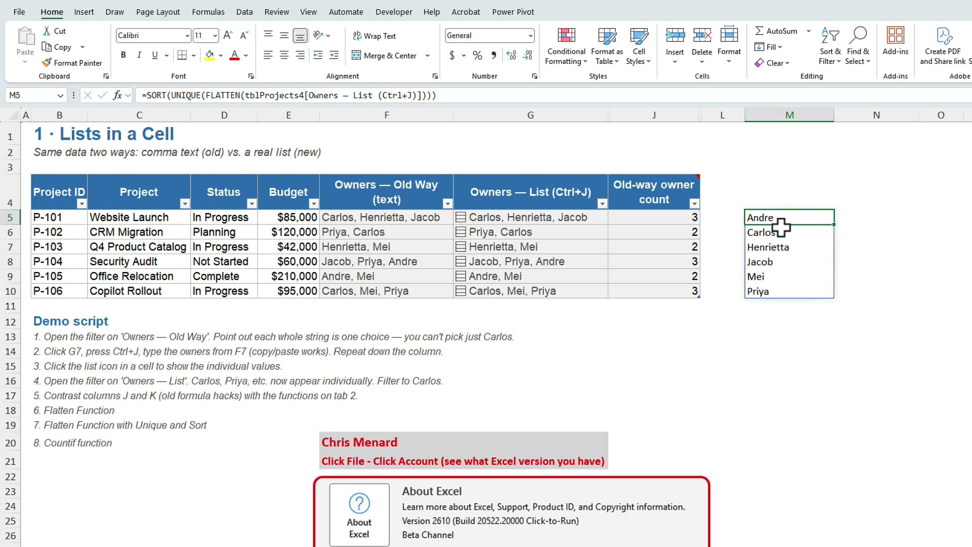

Excel SORT UNIQUE FLATTEN formula in the formula bar returning six sorted names: Andre, Carlos, Henrietta, Jacob, Mei, Priya — SORT, UNIQUE, and FLATTEN together return a clean, alphabetical list of every owner in the table.

Count each name with COUNTIF

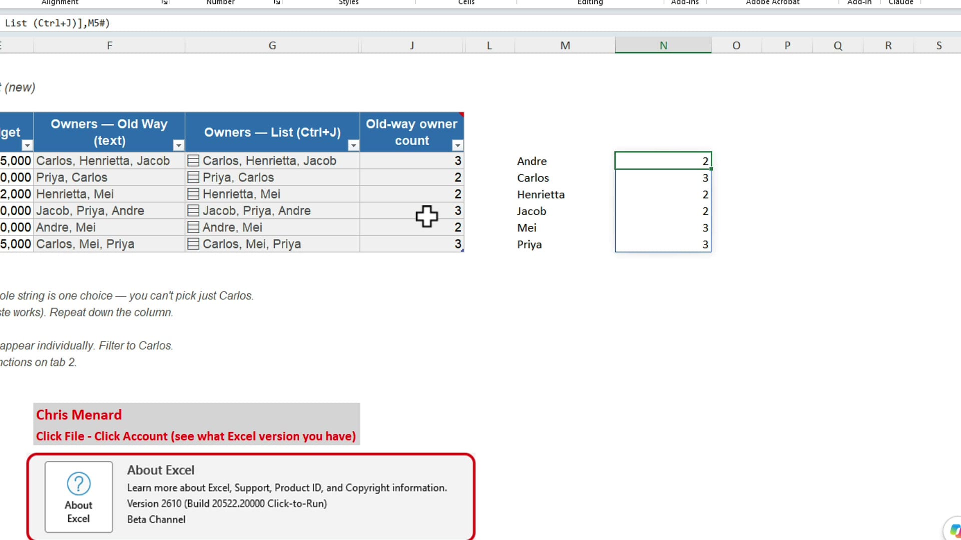
Next, count how many times each name appears. COUNTIF works directly against the list column. The first argument is the list column, and the second argument is the cell holding the unique names, M5, followed by a hashtag:

=COUNTIF(tblProjects4[Owners — List (Ctrl+J)],M5#)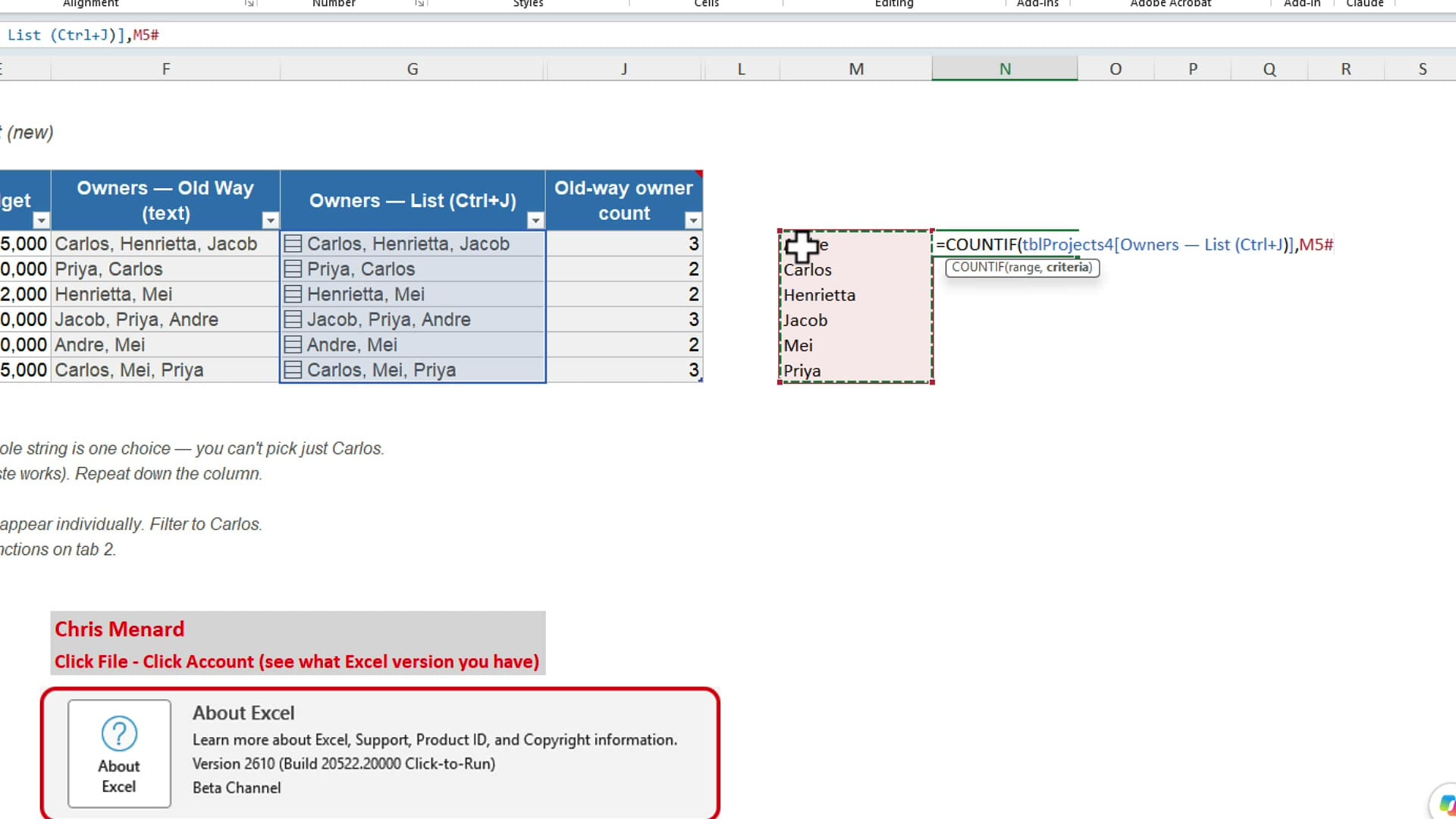

Excel COUNTIF formula being typed with the list column as the range and M5# as the criteria, with the spilled names outlined — Notice the hashtag after M5. It tells COUNTIF to use the entire spilled range of names, however long it gets.

The hashtag is the spill reference. It says "use everything that spilled from M5," so the counts fill down for every name with one formula. If you have paired UNIQUE, SORT, and COUNTIF before, this is the same pattern. The difference is that it now works on cells holding several values each.

Excel summary showing Andre 2, Carlos 3, Henrietta 2, Jacob 2, Mei 3, Priya 3 next to the project table — One formula, six counts. Carlos is three and Jacob is two, matching the conditional formatting check.

Test it with a new name

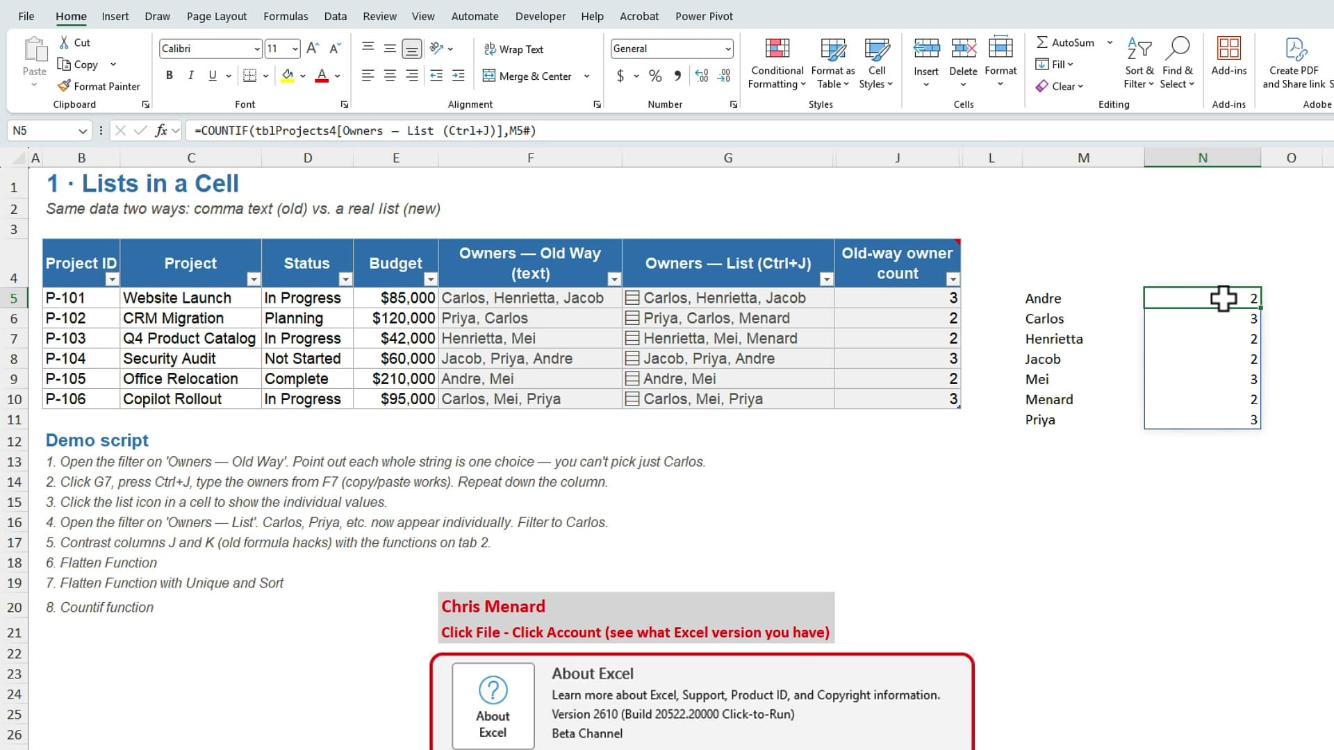
What is nice about this is that everything updates on its own. To prove it, I edit one of the list cells and add my last name, Menard. Menard shows up in the summary in alphabetical position with a count of one. Add Menard to a second project and the count goes to two. There is no formula to edit and no range to extend.

Excel list column with Menard added to two projects and the summary showing a new Menard row with a count of 2 — Add a name to any list and the summary picks it up: a new row for Menard, and the count updates as the name is added to more projects.

Lists, FLATTEN, and what to try first

I absolutely love this feature. One cell can hold several items, each item is filterable on its own, and FLATTEN with SORT, UNIQUE, and COUNTIF turns a column of lists into a live summary. If you are on the Beta Channel, take a column of comma-separated names, select it, press Ctrl + J, and open the filter dropdown. There is even more to lists than what I covered here, so I am breaking it up into several tutorials.