Microsoft Excel

Excel FILTER with UNIQUE and TRANSPOSE: Build Dynamic Lists

Turn a flat list of names and departments into a column per department that updates on its own. UNIQUE pulls the distinct departments, TRANSPOSE turns them into headers, and FILTER drops the right names underneath each one.

Here is a problem I run into often: I have one flat list of employees with a department next to each name, and what I really want is a column for each department with the right people underneath it. HR in one column, Accounting in the next, and so on — built once, updating on its own as the source list changes.

Three functions do the whole job: UNIQUE pulls the distinct department names, TRANSPOSE turns that vertical list into horizontal headers, and FILTER — one of my favorite Excel functions — drops the matching names underneath each one. No sorting, no copying, no manual cleanup.

The sample data

Excel Filter function with unique and transpose

Download the file used in this video and practice for yourself.

Excel Filter function with unique and transpose.xlsx

16 KB

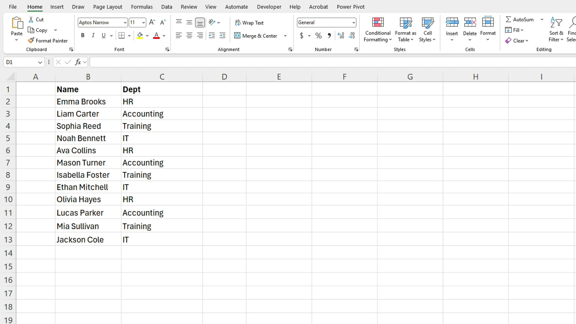
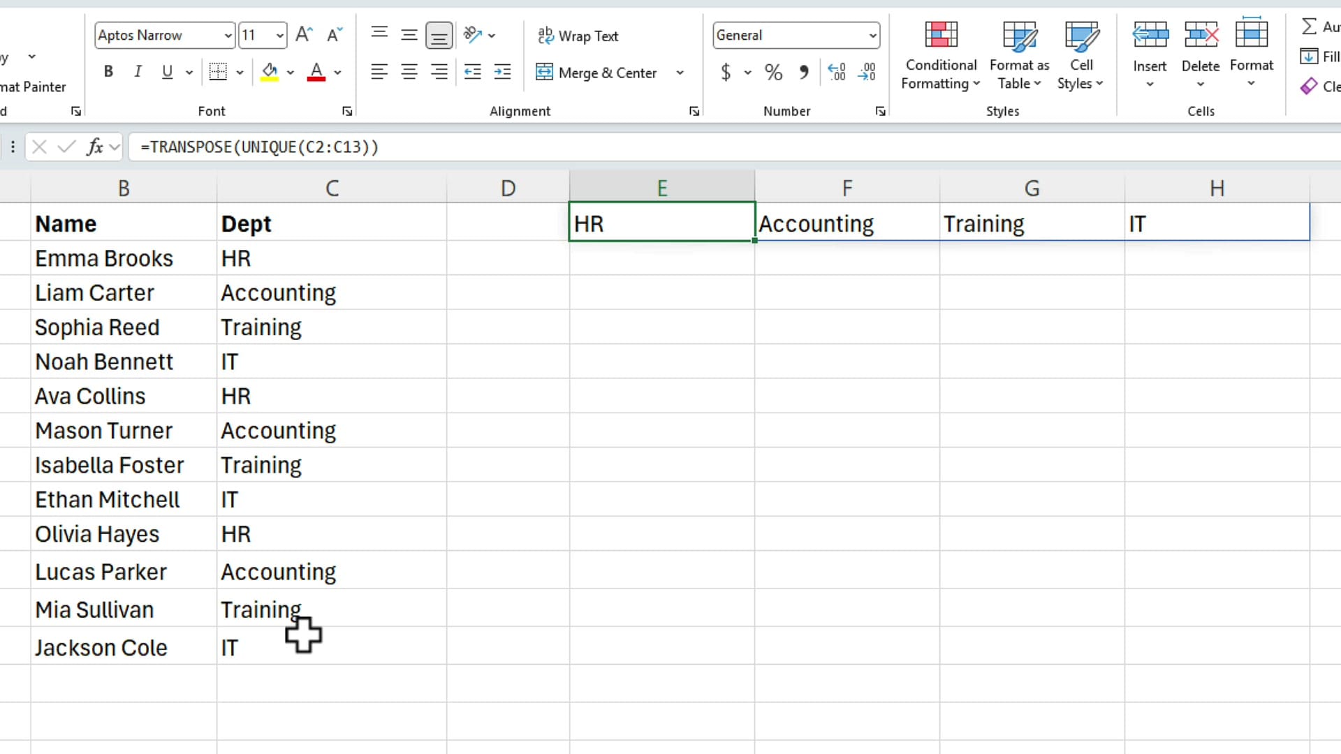
Column B has twelve names and column C has the department each person belongs to, in rows 2 through 13. There are four departments in that list — HR, Accounting, Training, and IT — but they repeat all the way down, and they are not in any particular order.

The layout I am building starts in cell E1. Row 1 gets the department names running across, and everything from row 2 down gets the people who belong to that department.

Excel worksheet with employee names in column B and department names in column C, rows 2 through 13 — The starting data: names in column B, departments in column C. The four departments repeat throughout the list.

Step 1: Get the distinct departments with UNIQUE

The UNIQUE function takes a range and hands back each value one time. Point it at the department column:

=UNIQUE(C2:C13)

Press Enter and there they are — HR, Accounting, Training, IT. Four departments out of twelve rows, no duplicates.

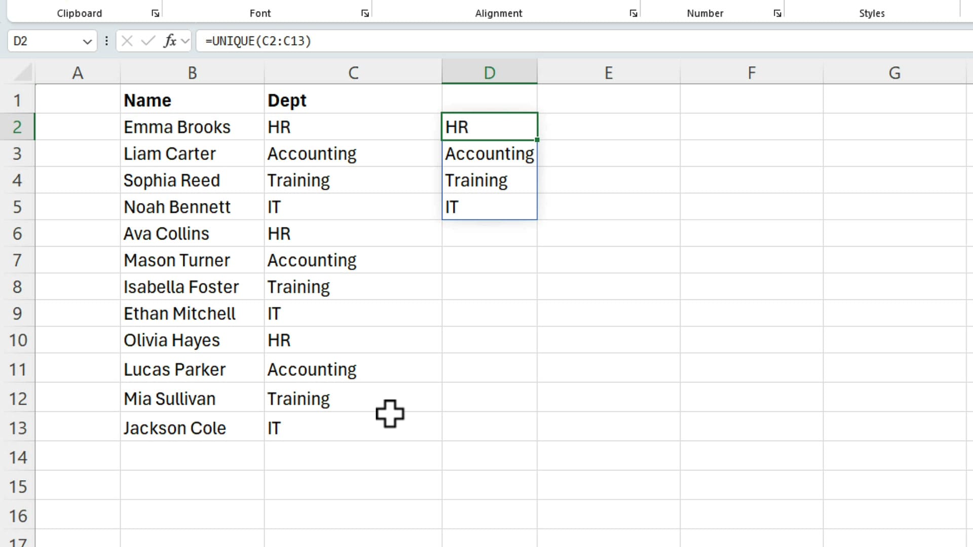
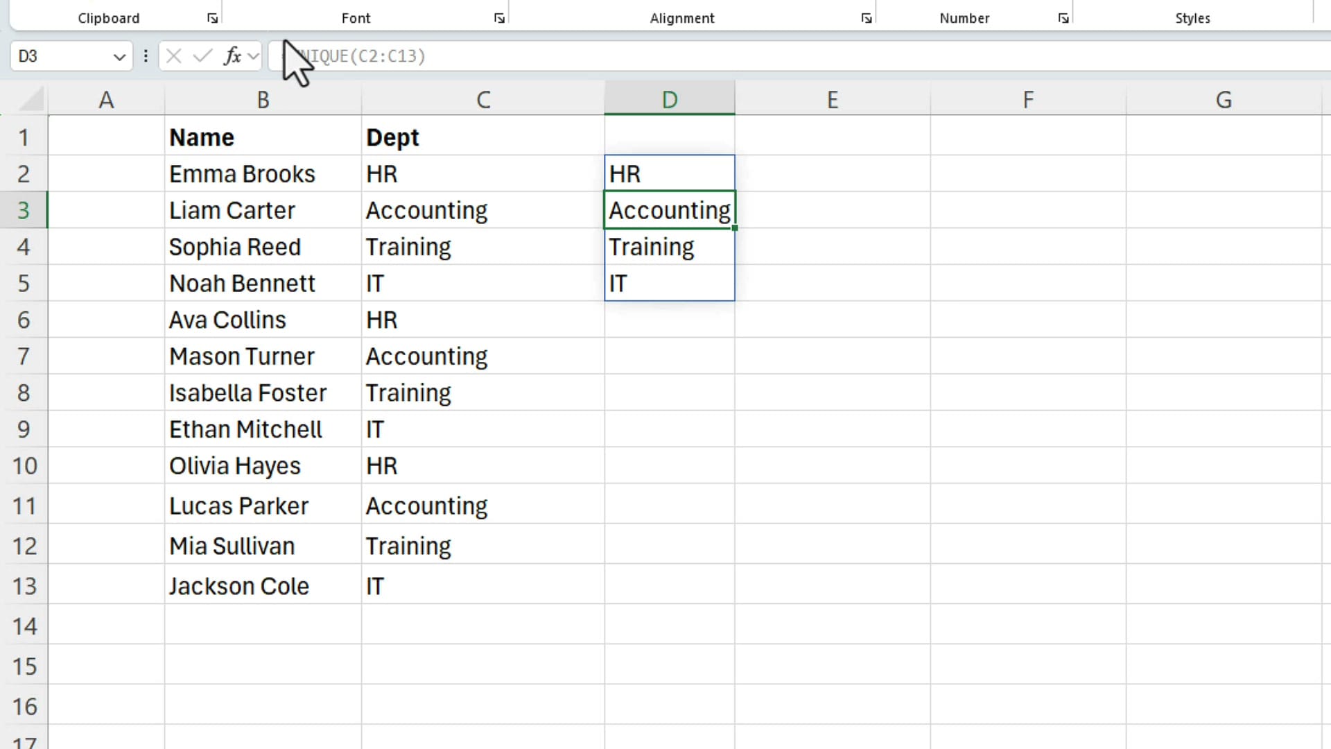
The UNIQUE function in cell D2 returning four distinct department names spilled down column D — =UNIQUE(C2:C13) returns the four distinct departments, spilled down the column.

One thing worth pointing out about dynamic arrays: the formula lives in a single cell. Click on the second result and the formula bar shows the text grayed out. That is Excel telling you the value is part of a spill range owned by the cell above it — you cannot edit it there.

Clicking a cell inside the UNIQUE spill range shows the formula grayed out in the formula bar — Click into the spill range and the formula appears grayed out. Only the top-left cell holds the actual formula.

Step 2: Turn the list sideways with TRANSPOSE

UNIQUE gave me exactly what I asked for, but it gave it to me going straight down, and I need my headers going left to right. TRANSPOSE flips a range from vertical to horizontal, and it nests around UNIQUE without any extra work.

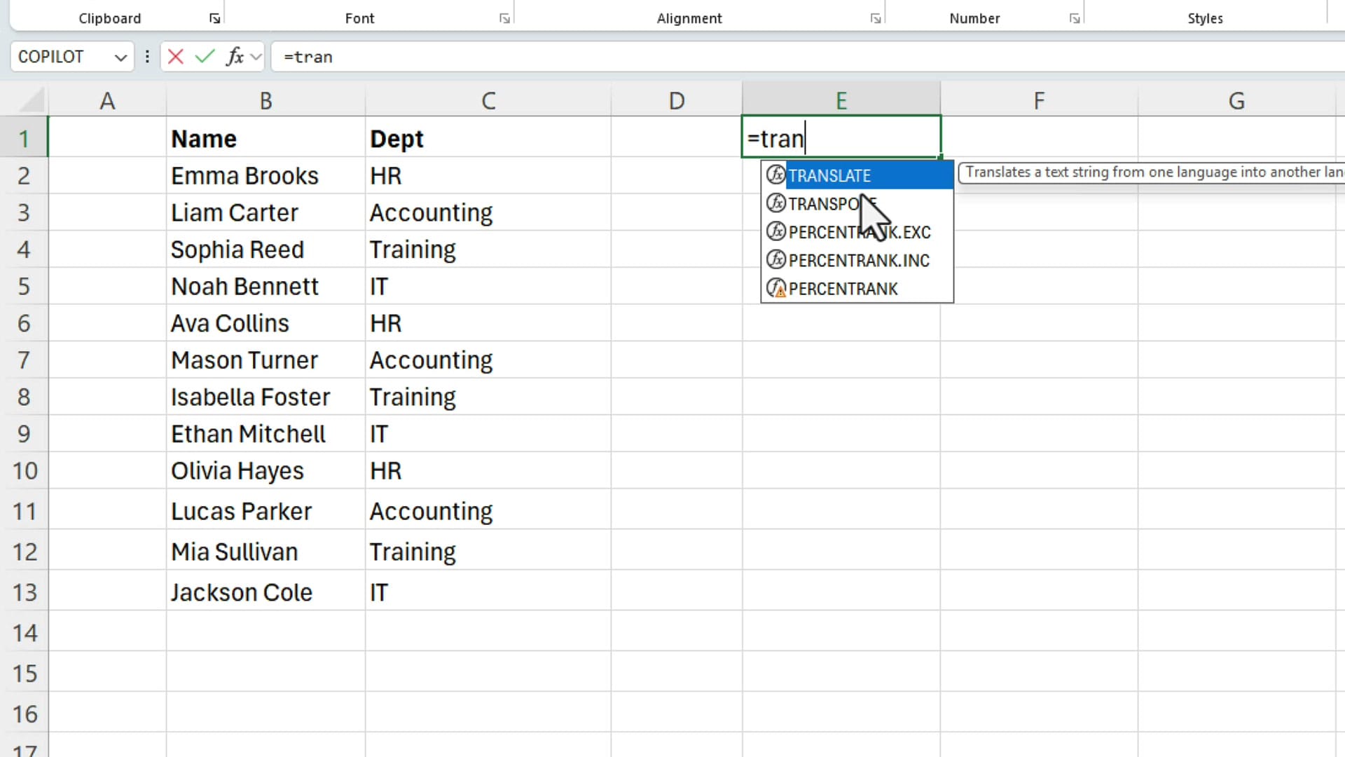
Start typing =TRAN in cell E1 and Excel offers TRANSLATE first, then TRANSPOSE — make sure you pick the second one.

Typing =TRAN in Excel showing the function autocomplete list with TRANSLATE and TRANSPOSE — TRANSLATE sits above TRANSPOSE in the autocomplete list, so watch which one you select.

Wrap TRANSPOSE around the UNIQUE formula and highlight the same department range:

=TRANSPOSE(UNIQUE(C2:C13))

Press Enter and the four departments spill across E1 through H1 instead of down. I made them bold so they read as headers, but that is cosmetic — the formula is doing the work.

TRANSPOSE wrapped around UNIQUE spilling the four department names horizontally across cells E1 through H1 — =TRANSPOSE(UNIQUE(C2:C13)) spills the departments across row 1 instead of down a column.

Step 3: Pull the names with FILTER

Now for the function I genuinely love. The FILTER function takes two required arguments: the array you want back, and the condition that decides which rows qualify.

Go to cell E2, directly under the HR header. Argument one is what I want to pick up — the names, B2:B13.

Typing the FILTER function in Excel with B2:B13 selected as the array argument and the tooltip showing array, include, if_empty — The FILTER tooltip shows the three arguments. Array is what comes back; include is the condition.

Argument two is what to include. I am testing the department column against whatever department is sitting in the header cell above:

=FILTER(B2:B13,C2:C13=E1)

Press Enter and I get Emma Brooks, Ava Collins, and Olivia Hayes. Always check what a formula is doing before you trust it — scan back through column C, find every row tagged HR, and confirm those are the same three people.

FILTER returning Emma Brooks, Ava Collins, and Olivia Hayes under the HR header, with the matching HR rows outlined in the source data — Three names come back under HR, and they match the three HR rows in the source data exactly.

Notice that the array and the condition point at two different columns. I am returning names from column B while testing departments in column C. That is the part that makes FILTER so useful — what you get back and what you test do not have to be the same range.

Step 4: Lock the references before you fill across

The formula is correct for HR, but it will fall apart the moment I drag it to the right, because B2:B13 and C2:C13 will shift over to C and D. Those two ranges need to stay put.

Double-click cell E2 to edit the formula, put your cursor in each range, and press the F4 function key to make it absolute:

=FILTER($B$2:$B$13,$C$2:$C$13=E1)

Editing the FILTER formula in Excel with F4 applied so the ranges read $B$2:$B$13 and $C$2:$C$13 — F4 locks both ranges with dollar signs so they do not shift when the formula moves across.

The E1 reference is different. That one should move — when the formula lands in F2 it needs to look at F1, in G2 at G1, and so on. So leave it relative and it works fine on its own.

If you want to be strict about it, you can press F4 twice to get a mixed reference, E$1. That freezes row 1 while leaving the column free to move. It is not necessary here, but it is a little cleaner, and it protects you if the formula ever gets copied down instead of across.

The FILTER formula edited to use the mixed reference E$1, freezing row 1 but not the column — F4 twice gives you E$1 — row 1 is frozen, the column is still free to move across.

Step 5: Fill the formula across

Select E2, grab the fill handle in the bottom-right corner, and drag across to H2. Let go, and every department fills in with its own people underneath it.

The finished Excel layout with four department headers across row 1 and the matching employee names filled underneath each one — One fill across and every department has its own column of names, all driven by formulas.

Because every cell here is a formula, the whole layout is live. Add a new hire to the bottom of the source list and their name appears under the right department. Add a brand new department and TRANSPOSE widens the header row automatically — you only need to fill the FILTER formula one column further.

The three formulas

=UNIQUE(C2:C13) — the distinct values from a column, each one listed once.
=TRANSPOSE(UNIQUE(C2:C13)) — the same list flipped from vertical to horizontal.
=FILTER($B$2:$B$13,$C$2:$C$13=E$1) — the names whose department matches the header above, ready to fill across.

UNIQUE, TRANSPOSE, and FILTER are all part of Excel's dynamic array family, so they spill onto the sheet and recalculate as the data underneath them changes. If you want to go further with the same building blocks, you can count how many people land in each group with COUNTIF, or use UNIQUE to find and remove duplicates in a messy list. Thank you for your time, and thank you for supporting my YouTube channel.