Microsoft Excel

Excel FILTER Function: Filter and Sort Data with Ease

The FILTER function spills back only the rows that match a condition. Three worked examples: filter by quantity, combine SORT with FILTER for sorted results, and build a between filter with two conditions.

The FILTER function in Excel is one of my favorite functions. Give it a range and a condition, and it spills back only the rows that match — no manual filtering, no copy-paste, and the results update automatically when your data changes.

Before we start, check your version. If you have Microsoft 365, Excel for the web, Excel 2021, or Excel 2024, you have the FILTER function. If you are using Excel 2019 or 2016, you will not see this function when you type it — it simply is not there.

The sample data

Excel Filter Function 01 20260705

Excel Filter Function 01 20260705.xlsx

17 KB

In columns A and B, I have a list of fictitious products and the quantity we have on hand — 25 products in rows 2 through 26. I am going to work through three examples with this data: products with a quantity less than 10 showing both columns, the same filter showing just the product names, and a "between" filter that picks up quantities from 5 to 15.

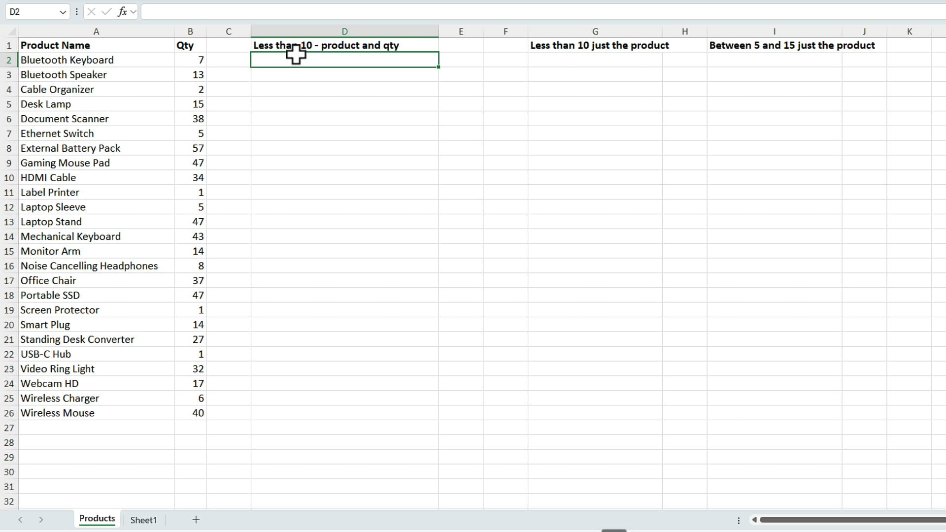
Excel worksheet with product names in column A, quantities in column B, and headers for three FILTER examples — The sample data: 25 products with quantities, and three FILTER challenges laid out across the top.

Example 1: Filter products with a quantity less than 10

I want to find the products that are less than ten in quantity, and in this first example, I want to show both the product and the quantity. The FILTER function takes three arguments, and the first two are required:

array — what do you want to pick up? I am going to select A2:B26, both columns.
include — what do you want to include? Quantity less than ten: B2:B26<10.
[if_empty] — optional; what to return if nothing matches.

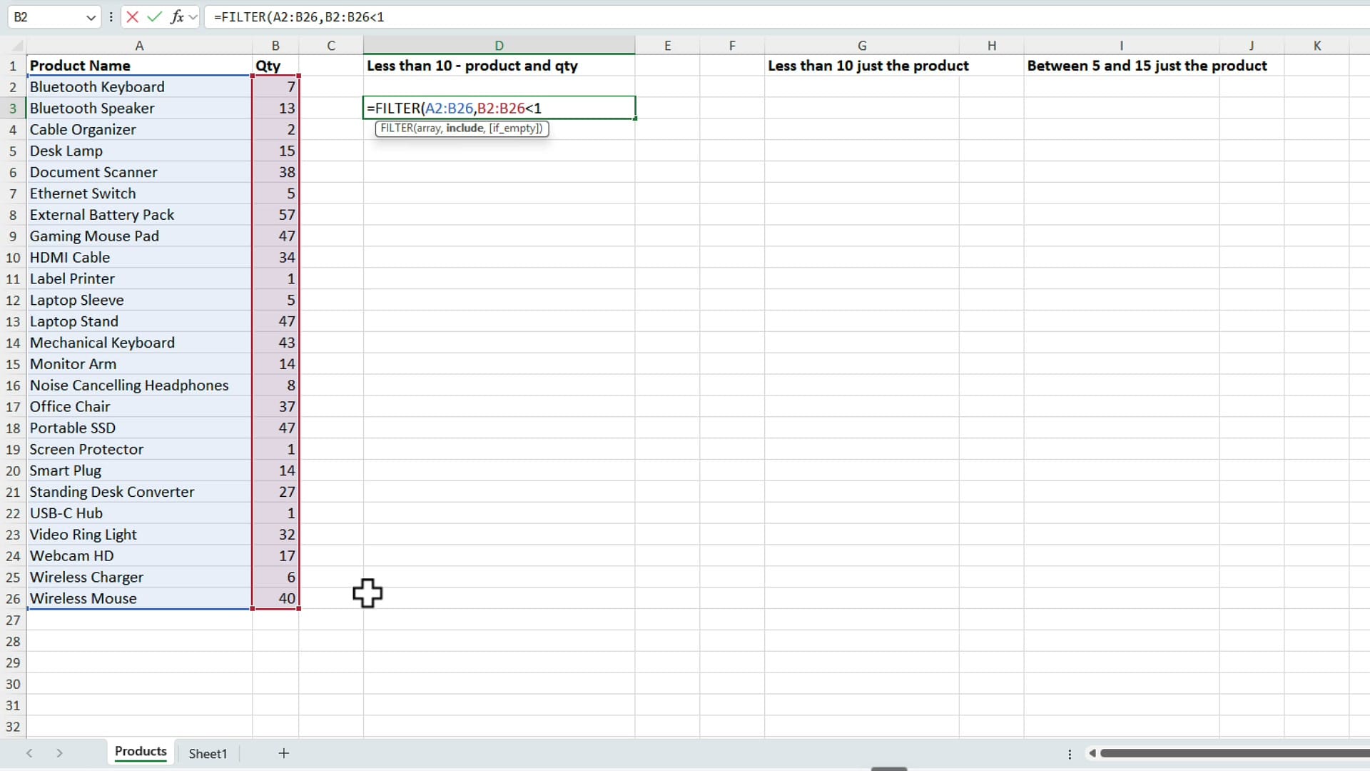
Typing the FILTER function in Excel with the tooltip showing the array, include, and if_empty arguments — As you type, Excel's tooltip shows the three arguments: array, include, and the optional if_empty.

The finished formula:

=FILTER(A2:B26,B2:B26<10)

Press Enter, and there are your answers — every product with fewer than ten units, spilled into two columns.

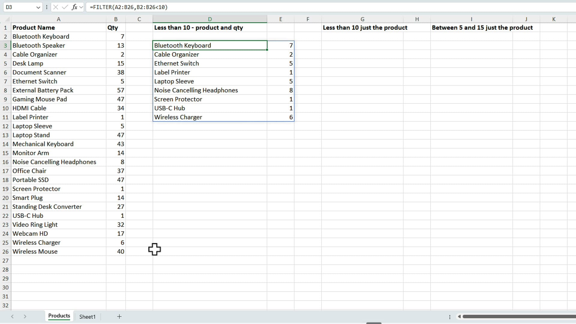
FILTER function results showing nine products with quantities under ten in two spilled columns — One formula returns every product under ten units, with its quantity, in a spilled range.

If you want to test the results, go over to column B and do a sort, smallest to largest. Every quantity less than ten in the source data is a perfect match with the filtered list on the right.

Bonus tip: Combine SORT with FILTER

Here is a bonus tip: you can include sorting right inside the same formula. Edit the function and wrap the SORT function around FILTER:

=SORT(FILTER(A2:B26,B2:B26<10))

Now the results are sorted by product name — SORT defaults to the first column, ascending.

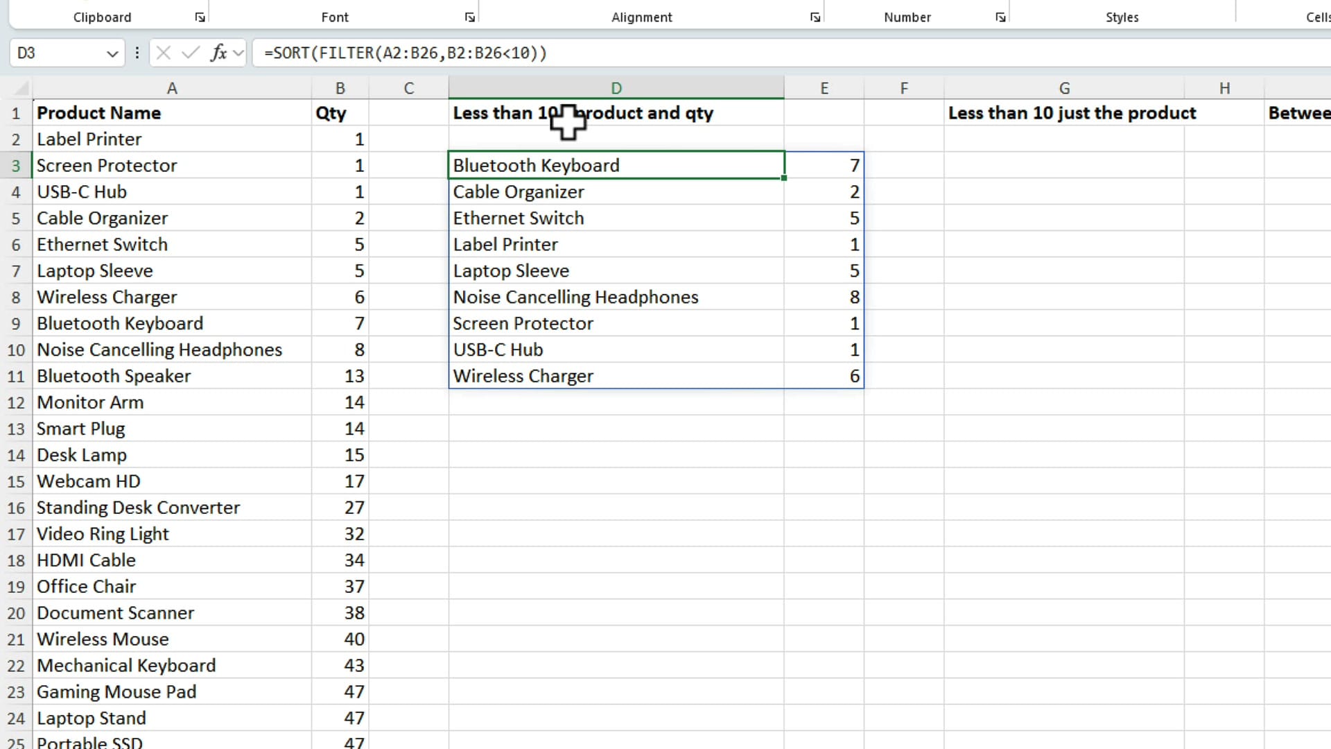
SORT wrapped around FILTER in Excel sorting the filtered results by product name — Wrap SORT around FILTER and the spilled results come back sorted by the first column — product name.

If you would rather sort by the quantity, tell SORT which column to use. Since I picked up two columns in the FILTER function, quantity is column 2, so the sort index is 2. By default that sorts smallest to largest. To flip it largest to smallest, add a -1 for descending as the next argument:

=SORT(FILTER(A2:B26,B2:B26<10),2,-1)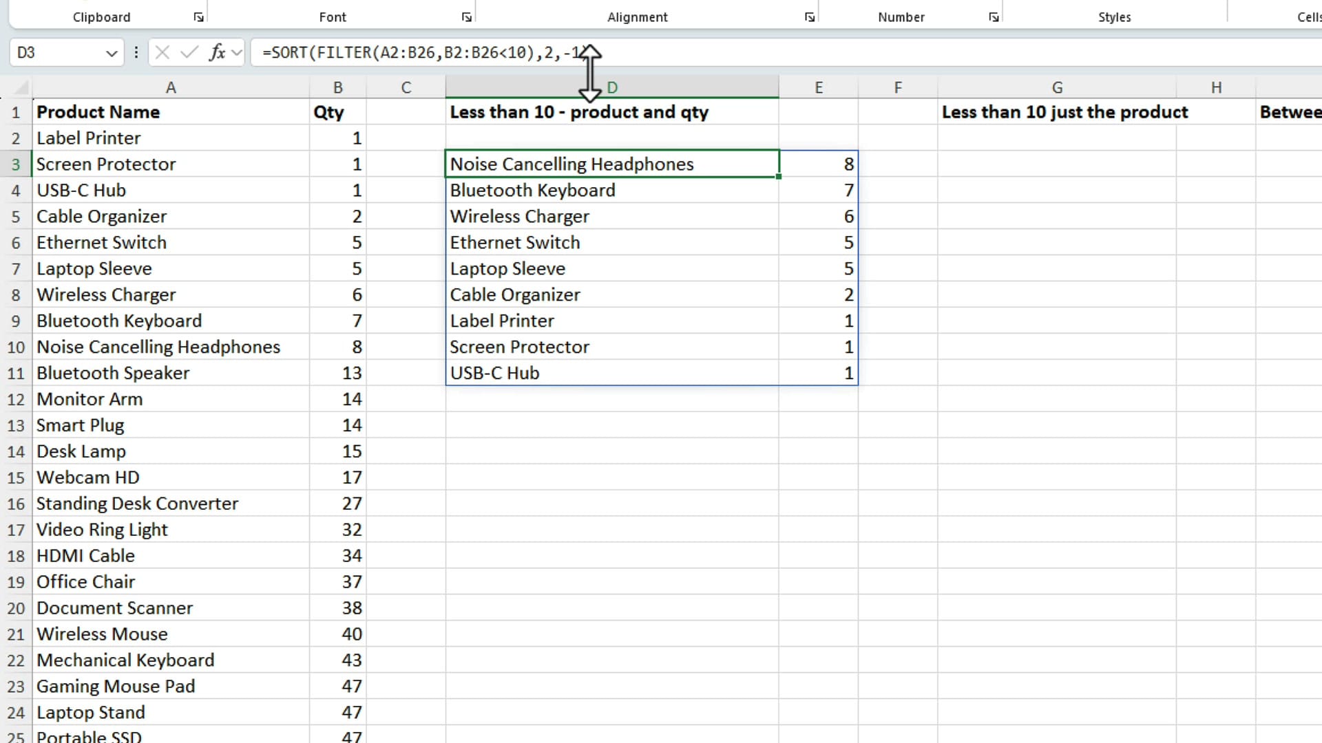

SORT and FILTER combined with a sort index of 2 and -1 for descending order by quantity — Sort index 2 targets the quantity column, and -1 flips the order to descending — highest quantities first.

Example 2: Show just the products

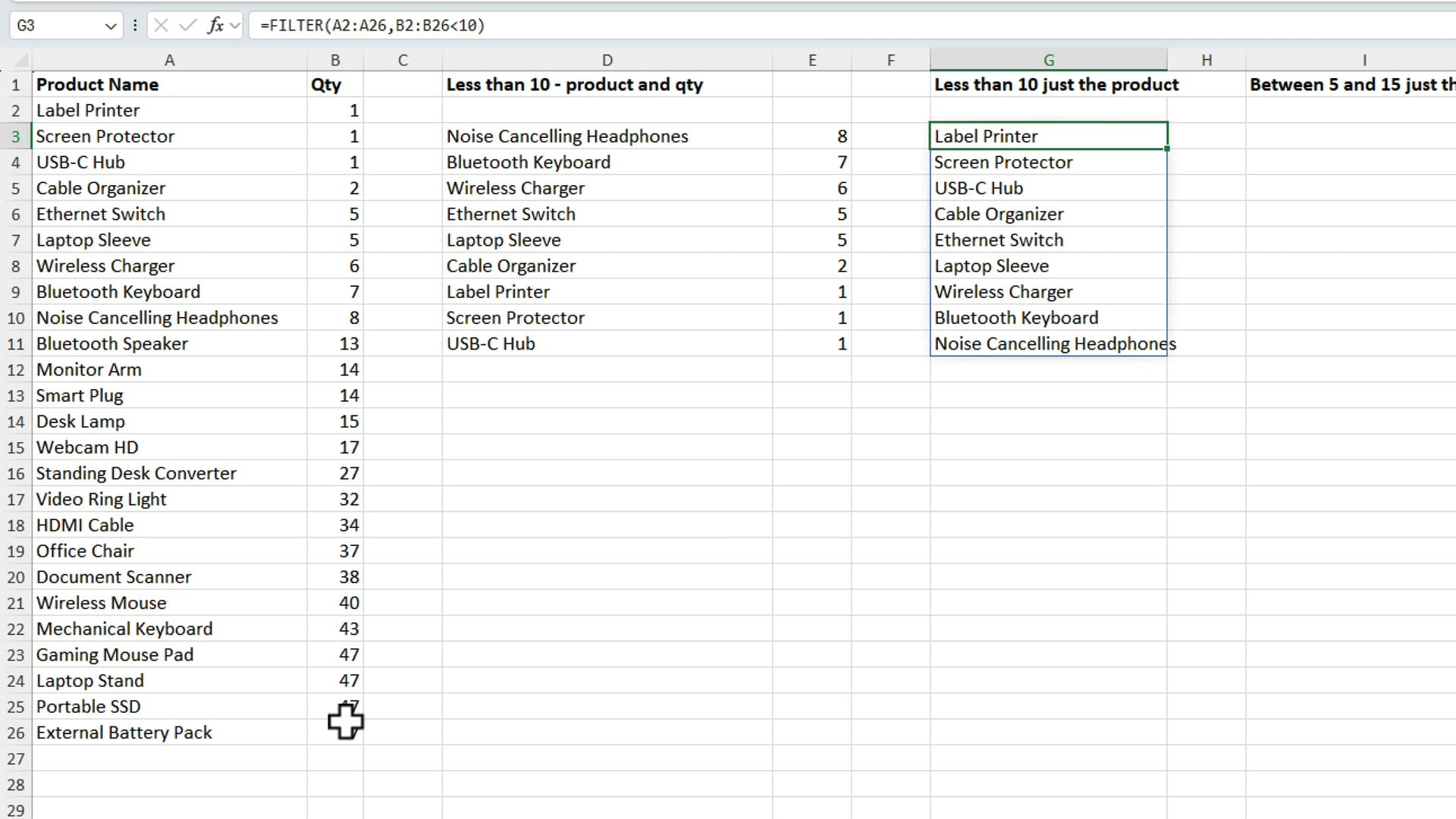
Someone says, "Just show me the products — I do not want the quantity." Same filter, different array. Instead of picking up columns A and B, I am just going to pick up A2:A26. The include argument stays exactly the same, because I am still testing the quantity column:

=FILTER(A2:A26,B2:B26<10)

There you go — just the product names, one column. That is the key idea: the array you return and the column you test do not have to be the same.

FILTER returning a single column of product names filtered by quantities in a different column — Return one column while testing another: the array is A2:A26, but the condition still checks B2:B26.

Example 3: Between two numbers (5 to 15)

For the third example, I want just the products again, but this time with a "between" condition: quantities from 5 through 15. This one is a little tricky, because FILTER does not have a built-in between — you build it with two conditions multiplied together:

=FILTER(A2:A26,(B2:B26>=5)*(B2:B26<=15))

The first condition is greater than or equal to 5, because I want to pick up the number five itself. The star (*) works as an AND — both conditions have to be true. The second condition is less than or equal to 15.

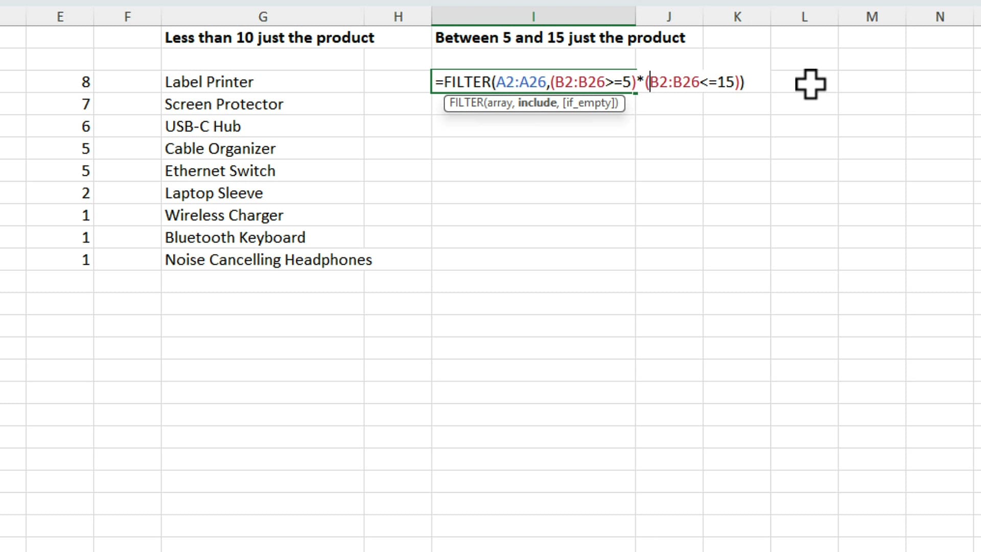
FILTER formula with two conditions multiplied together to create a between filter in Excel — The between pattern: two conditions in parentheses, joined with a star — Excel's array version of AND.

One gotcha to watch for: each condition needs its own set of parentheses. I almost made that mistake myself — I forgot the open paren before the second B2:B26, and the formula would not behave until I added it. If your between filter is not working, check the parentheses first.

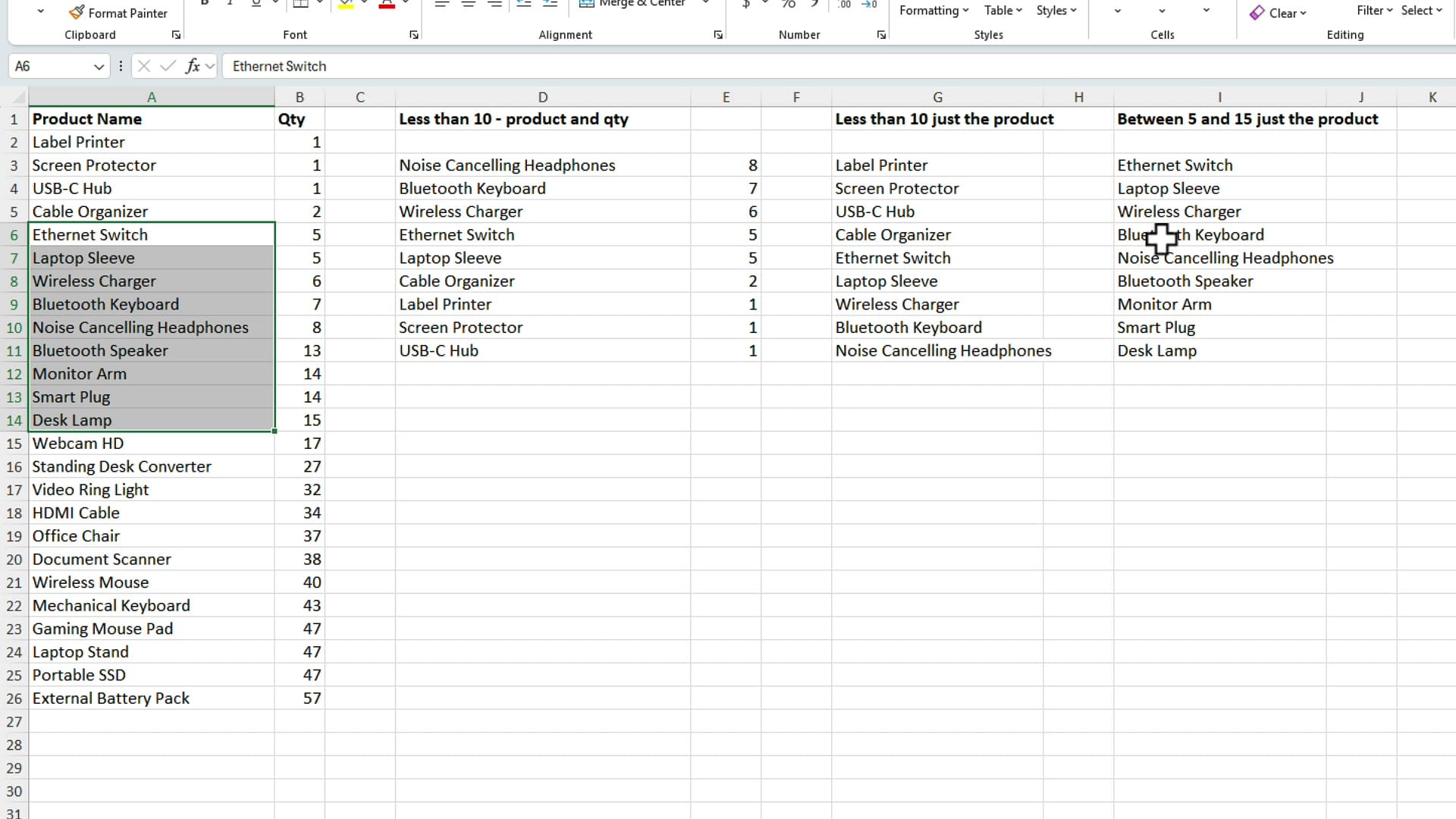
Let's do a quick check on the results. Highlight the quantities between 5 and 15 in the source data: nine items. The FILTER result: nine items. Perfect match.

All three FILTER examples complete, with the between filter returning nine products matching quantities from 5 to 15 — All three examples side by side, with the between filter returning exactly nine matching products — verified against the source data.

Recap

Three patterns cover most of what you will do with FILTER day to day:

=FILTER(A2:B26,B2:B26<10) — filter rows on a condition and return multiple columns.
=SORT(FILTER(...),2,-1) — wrap SORT around FILTER to sort the results, by any column, in either direction.
=FILTER(A2:A26,(B2:B26>=5)*(B2:B26<=15)) — multiply conditions for a between (AND) filter.

FILTER is part of Excel's dynamic array family, alongside functions like SORT and UNIQUE — they all spill results onto the sheet and recalculate as your data changes. I appreciate your time, and thank you for your support of my YouTube channel.