
Excel XLOOKUP: Why Tables Are Better Than Ranges for Lookups
The same XLOOKUP built two ways: against a plain range with absolute references, then against named tables with structured references. See why the table version survives new data without an edit.


There are a lot of reasons to convert a range into an Excel Table, but the one I lean on most at work has to do with lookups. Once your lookup data lives in a table, your formulas get shorter, you stop fighting with absolute references, and the formula keeps working when someone adds a row to the source data.
Here I am going to run the same task two ways. Method one uses a plain range. Method two — my preferred method — uses tables. Same data, same function, very different maintenance.
Why tables beat ranges
Before the walkthrough, here is the short list of what you get when you convert a range to a table:
| Feature | Benefit |
|---|---|
| Automatic expansion | New rows become part of the dataset automatically |
| Structured references | Formulas become easier to read |
| Automatic formatting | Consistent appearance |
| Built-in filtering and sorting | No setup required |
| Total Row | Quick SUM, COUNT, AVERAGE |
| Better PivotTables | Source grows automatically |
| Better charts | Charts expand as data grows |
| Better Copilot results | Copilot understands the dataset more effectively |
The first two are the ones that matter for lookups, and they are what the rest of this post demonstrates.
The sample data
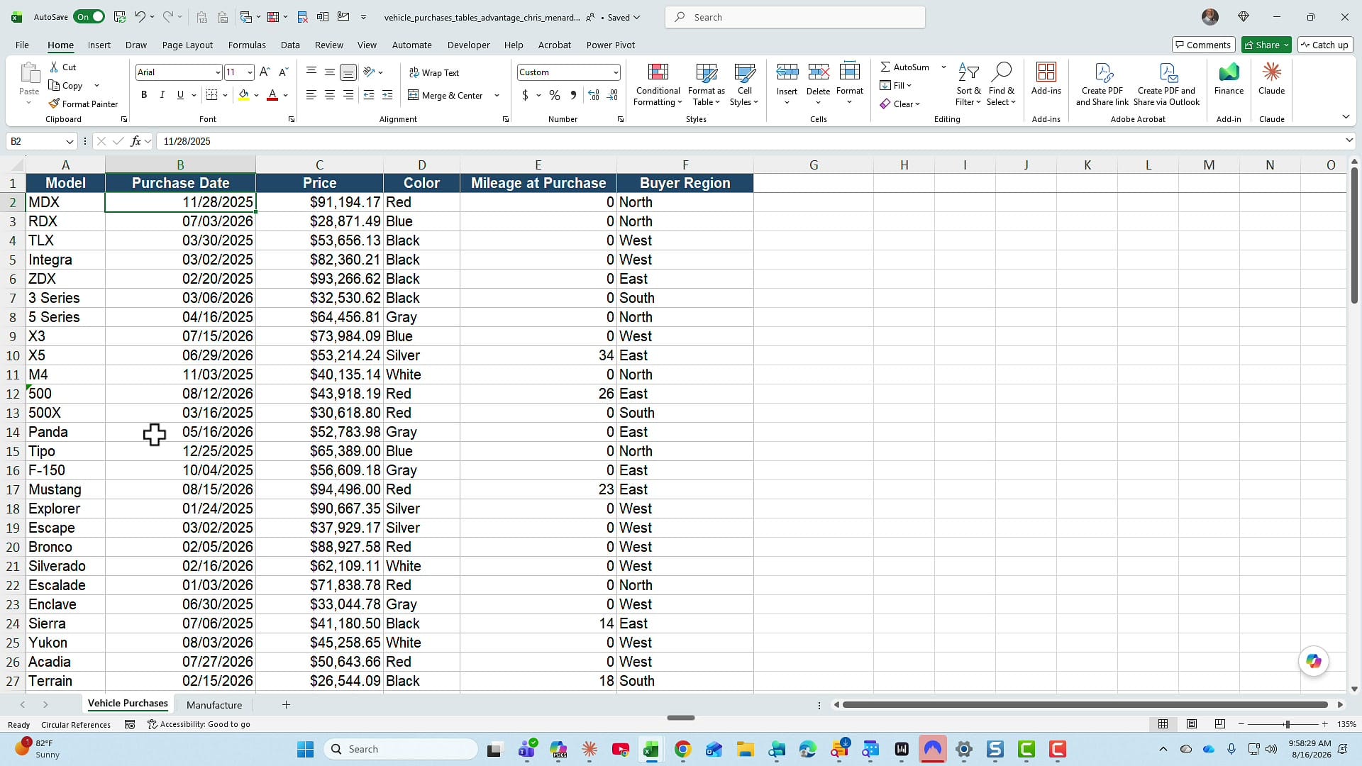
The workbook has two worksheets. Vehicle Purchases holds the transactions: the car model in column A, then purchase date, price, color, mileage at purchase, and buyer region. There are 95 records, in rows 2 through 96.
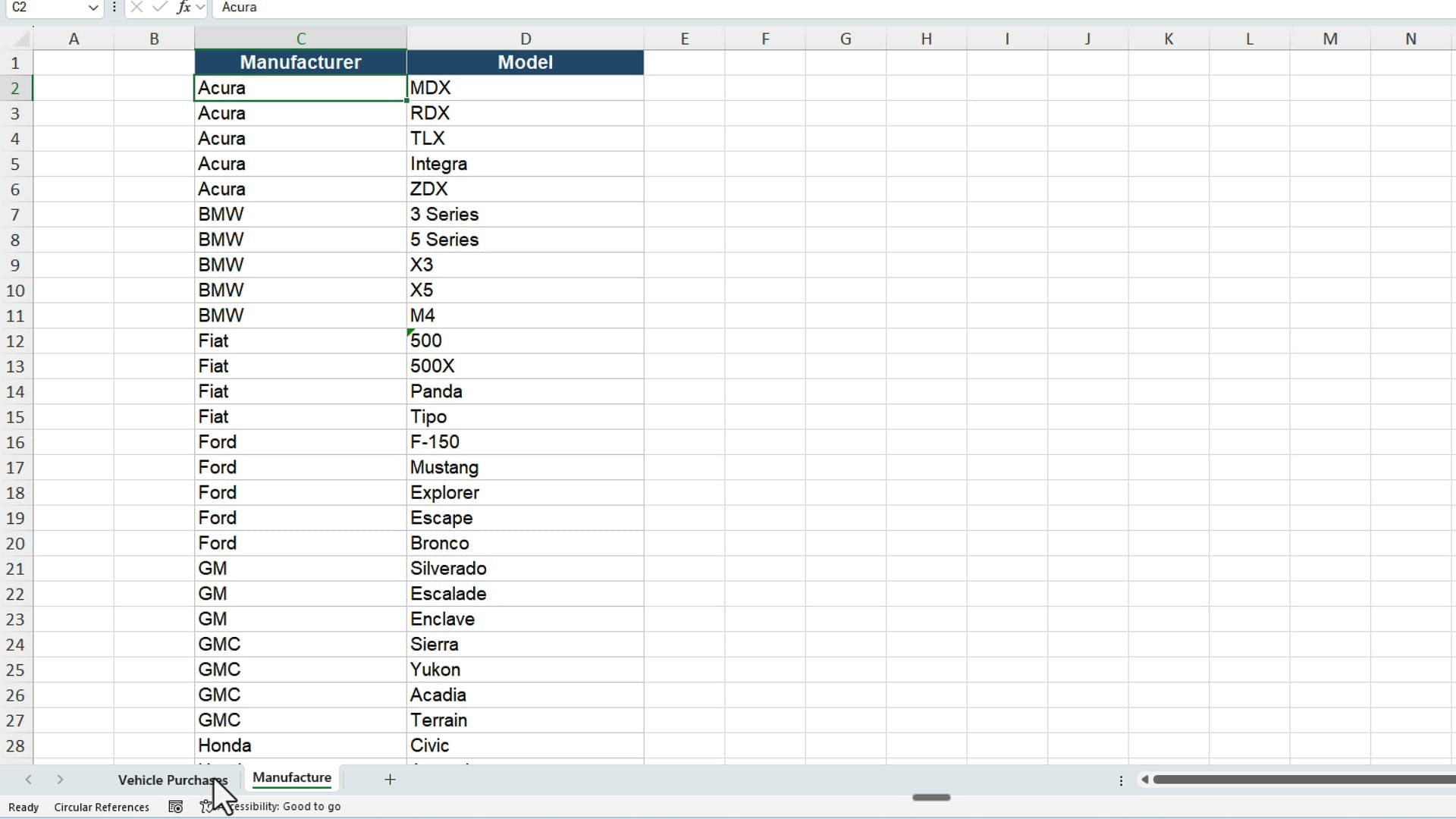
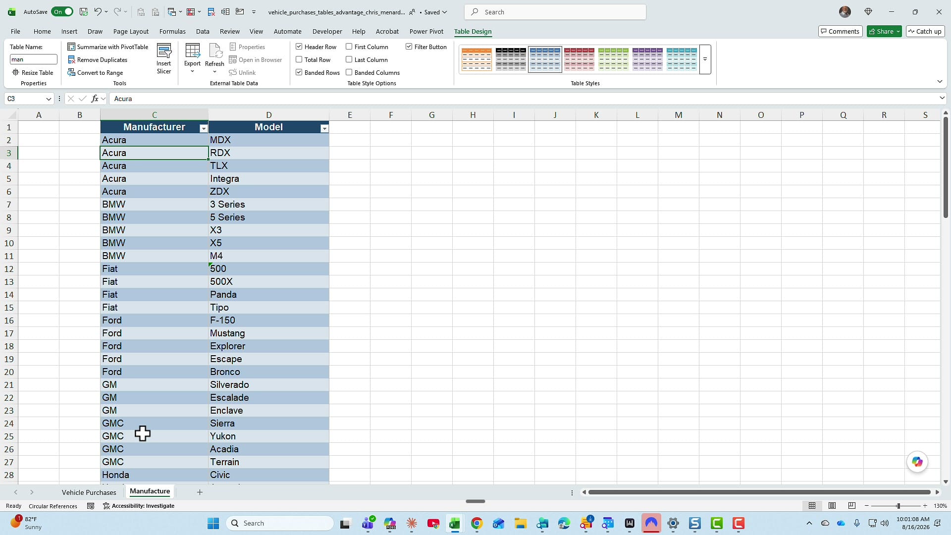
The second worksheet, Manufacture, is the lookup list. Column C has the manufacturer and column D has the model, again in rows 2 through 96. Notice the order: the value I am searching for (model) sits to the right of the value I want back (manufacturer). VLOOKUP cannot look left, which is one reason I use XLOOKUP for this.
Method 1: XLOOKUP against a range
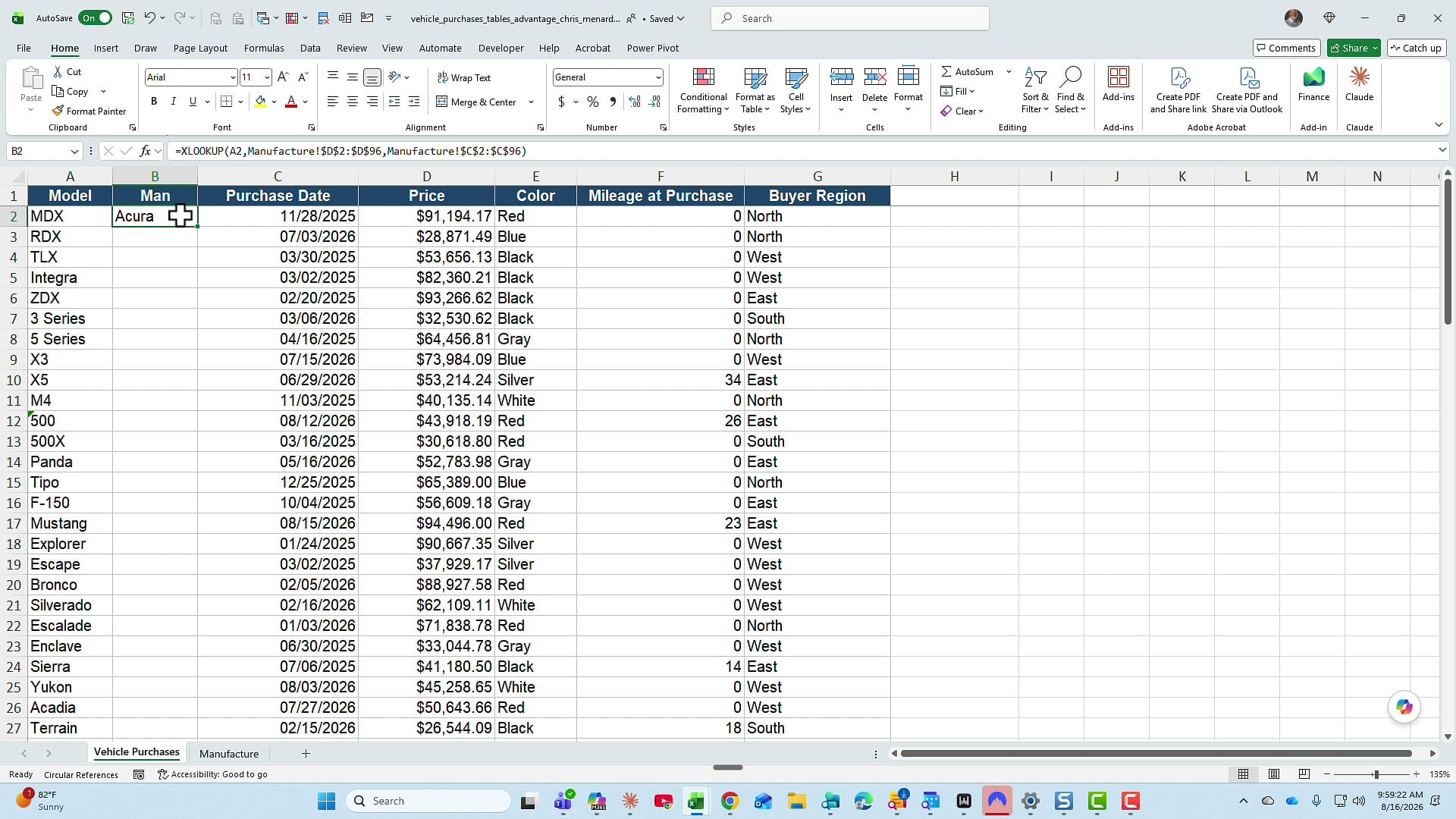
I inserted a column next to Model on the Vehicle Purchases sheet and called it Man, short for manufacturer. Then in B2 I built an XLOOKUP with three arguments:
- lookup_value — A2, the model on this row
- lookup_array — Manufacture!D2:D96, the model column on the other sheet
- return_array — Manufacture!C2:C96, the manufacturer column
Both of those ranges have to be locked down, or the references shift as the formula fills down. Press F4 right after selecting each range to cycle to an absolute reference — that is what turns D2:D96 into $D$2:$D$96.
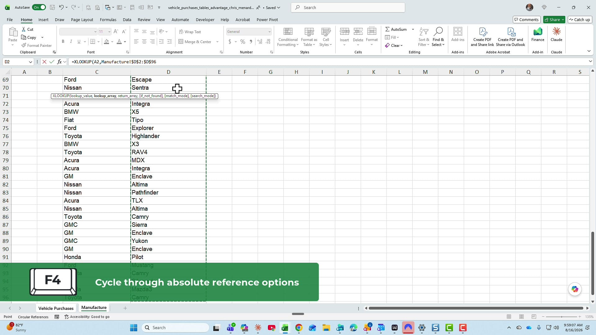
There is a small annoyance built into this method. After selecting the lookup array you are parked at the bottom of the sheet at row 96, so you have to scroll all the way back to the top to select the return array, then press F4 again. The finished formula:
=XLOOKUP(A2,Manufacture!$D$2:$D$96,Manufacture!$C$2:$C$96)Press Enter and B2 returns Acura, which is correct for an MDX. But the formula only exists in one cell, so I still have to fill it down — double-click the fill handle in the bottom-right corner of the cell to copy it to the bottom of the data.
The problem with a fixed range
None of that is a deal breaker. The real problem shows up the first time the source data grows.
Say a 4Runner purchase gets added as row 97. 4Runner is not in the manufacturer list yet, so filling the formula down returns #N/A. That part is expected — the fix should be to add 4Runner and Toyota to the Manufacture sheet.
So I add them, and they land in row 97 of the lookup list. Go back to Vehicle Purchases, and it still says #N/A. The formula's lookup range stops at row 96, so it never sees row 97. To fix it I have to go edit the formula and change every 96 to a 97.
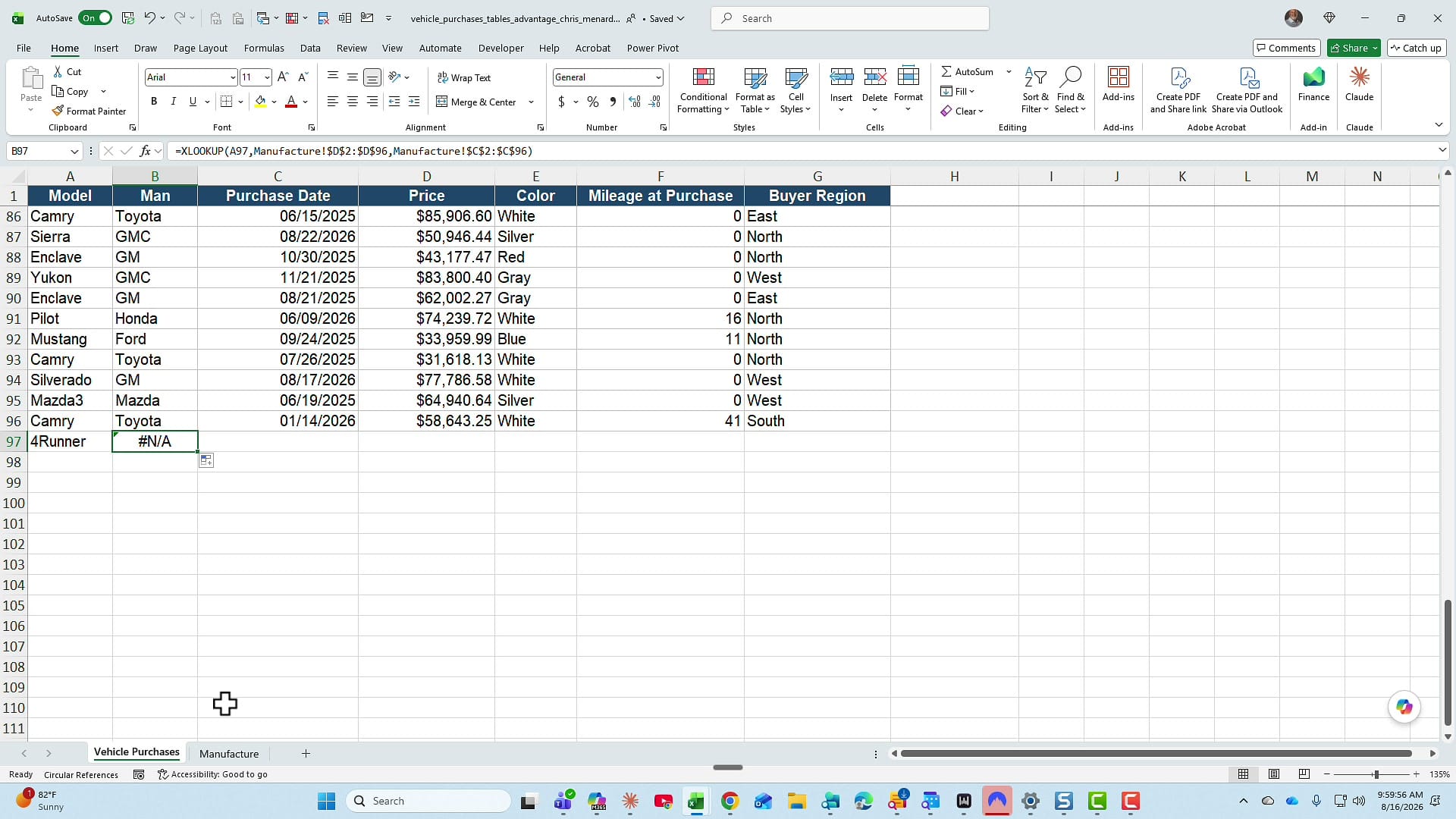
That is the maintenance tax on a fixed range. Every time the lookup list grows, someone has to remember to widen the formula — and if they forget, the error is quiet and easy to miss in a long column.
Method 2: Convert both ranges to tables
Starting over from scratch, this time the first thing I do is convert the data. Click anywhere inside the range and press Ctrl + T. Excel picks up the entire range automatically, and as long as your first row is headers, leave My table has headers checked and click OK.
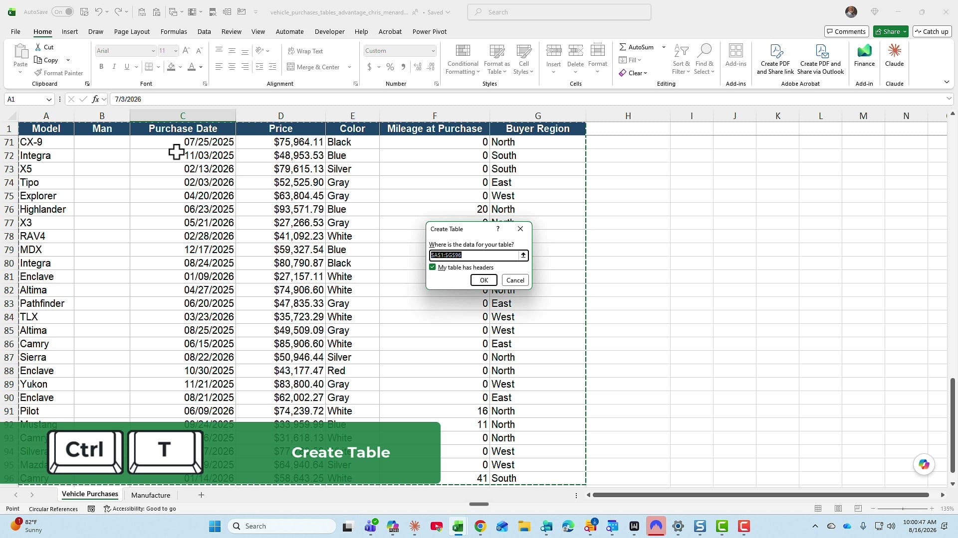
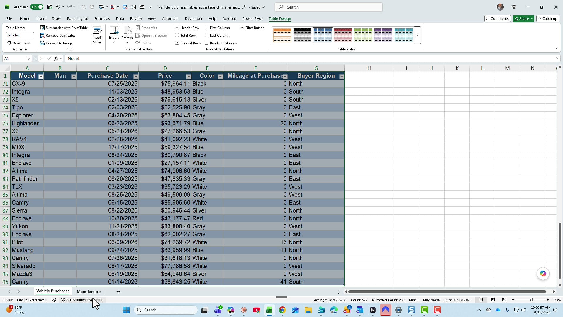
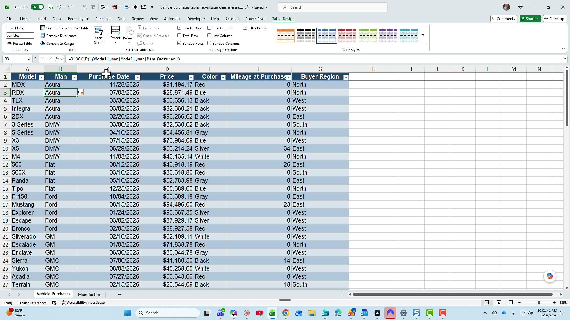
Naming the table is not required, but I always do it, because the name is what shows up in your formulas. With the cursor inside the table, go to the Table Design tab and type a name in the Table Name box. I named the purchases table vehicles.
Then do the same on the Manufacture sheet. Ctrl + T, confirm the headers, and name it. I used man — short names are easier to type inside a formula.
XLOOKUP with structured references
The function does not change — it is still XLOOKUP, with the same three arguments. What changes is how you point at the data. Instead of typing A2 for the lookup value, click the cell and Excel writes [@Model], which means "the Model column on this row." Instead of selecting D2:D96 and pressing F4, hover over the header of the Model column in the man table and click once. Same for the Manufacturer column.
=XLOOKUP([@Model],man[Model],man[Manufacturer])Compare that to the range version. It is shorter, it reads in plain English, and there is no F4 at all — structured references do not shift when the formula copies, so there is nothing to lock down. If you have Copilot available, structured references are also easier for it to work with; Copilot's formula completion writes XLOOKUP formulas more reliably when the source is a named table.
Press Enter, and here is the part I like most: the formula fills the entire column by itself. That is a calculated column — a table feature. No double-click on the fill handle, no dragging.
Now watch what happens when the data grows
Back to the 4Runner. Add 4Runner and Toyota to the man table, and the table expands to include the new row automatically — that is the automatic expansion from the list at the top. Because the formula points at man[Model] rather than a fixed D2:D96, it picks up the new row with no edit at all.
Return to the vehicles table and the 4Runner row now reads Toyota. Nothing to change, nothing to remember.
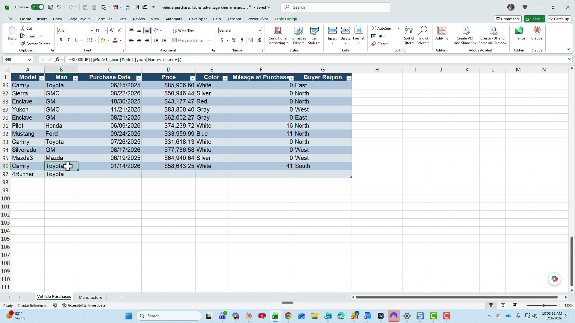
Add a new purchase row to the bottom of the vehicles table and you get the same behavior in the other direction — the table grows and the calculated column writes the formula into the new row for you.
Why I use tables for lookups
I do XLOOKUP constantly at work, and I am always doing it against tables. The formula is shorter, I skip the absolute references entirely, it fills down on its own, and it survives new data without anyone having to babysit a range. That last point is the one that saves real time — a formula nobody has to maintain is a formula that does not quietly break.
It pays off past lookups too. A table is a better PivotTable source, charts expand as the data grows, dynamic functions like FILTER stay accurate, and if you want to skip lookup formulas between sheets altogether, you can link tables through Excel's Data Model instead. For a walkthrough of the same cross-sheet XLOOKUP pattern in a different workbook, see this cross-sheet XLOOKUP example.
If your lookup data is still sitting in a plain range, press Ctrl + T on it. It takes two seconds, and you get all these benefits for free.
Related guides
 Chris Menard
 Chris Menard
 Chris Menard
 Chris Menard