Microsoft Excel

Excel PivotTables: How to Use Defer Layout Update

Working with a large data set? Turn on Defer Layout Update in the PivotTable Fields pane, arrange every field you need, and apply all the changes at once with a single click on Update.

When you build a PivotTable from a large data set, every field you check, uncheck, or drag triggers a recalculation. On a small workbook you never notice. On a big one, you wait after every single click. Defer Layout Update fixes that: you make all of your layout changes first, and Excel recalculates once, when you tell it to.

Defer Layout PivotTable - Chris Menard

Download example file and try this out

defer_layout_pivottable_menard_chris.xlsx

62 MB

The workbook I use here is 62 MB and has one million records, so it is a good test for this feature.

Start with a table

My data is already a table. I clicked inside it, pressed Ctrl + T, and named the table tbl_customers in the Table Name box on the Table Design tab. Basing your PivotTable on a table instead of a range means new rows get picked up when you refresh — here is why a table is the better PivotTable source.

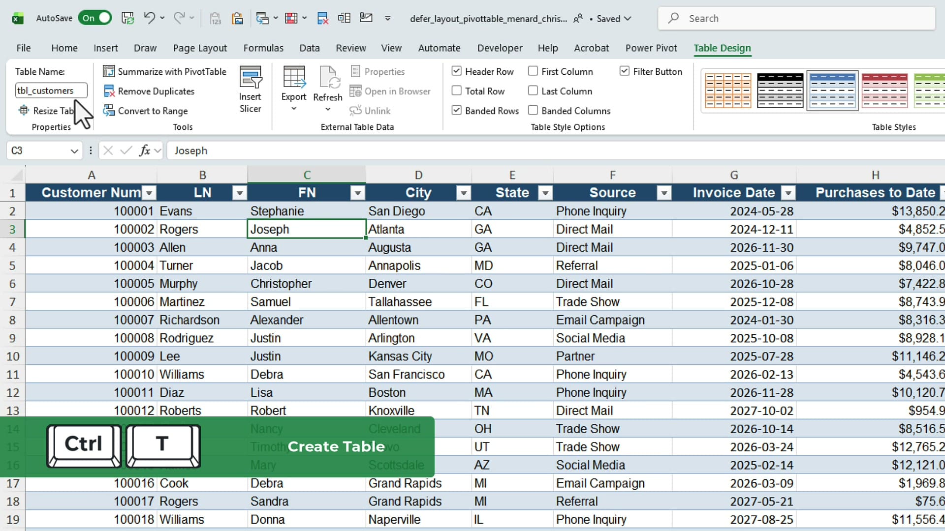
Excel customer data formatted as a table named tbl_customers on the Table Design tab, with a Ctrl+T Create Table keyboard callout — The source data is a table named tbl_customers, created with Ctrl + T.

For this example I am working with these fields:

State
City
Source
HouseholdType
Purchases to Date — the numeric field I will summarize

Create the PivotTable

With your cursor in the table, go to Insert > PivotTable. The Table/Range box already shows the table name. Leave New Worksheet selected and click OK.

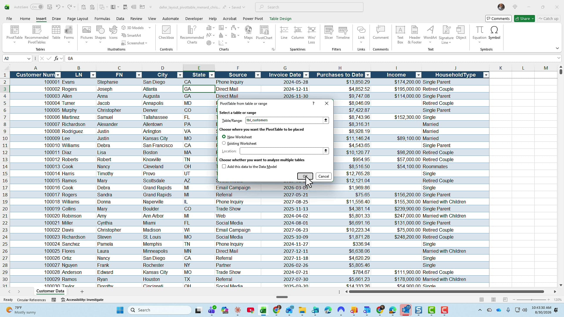
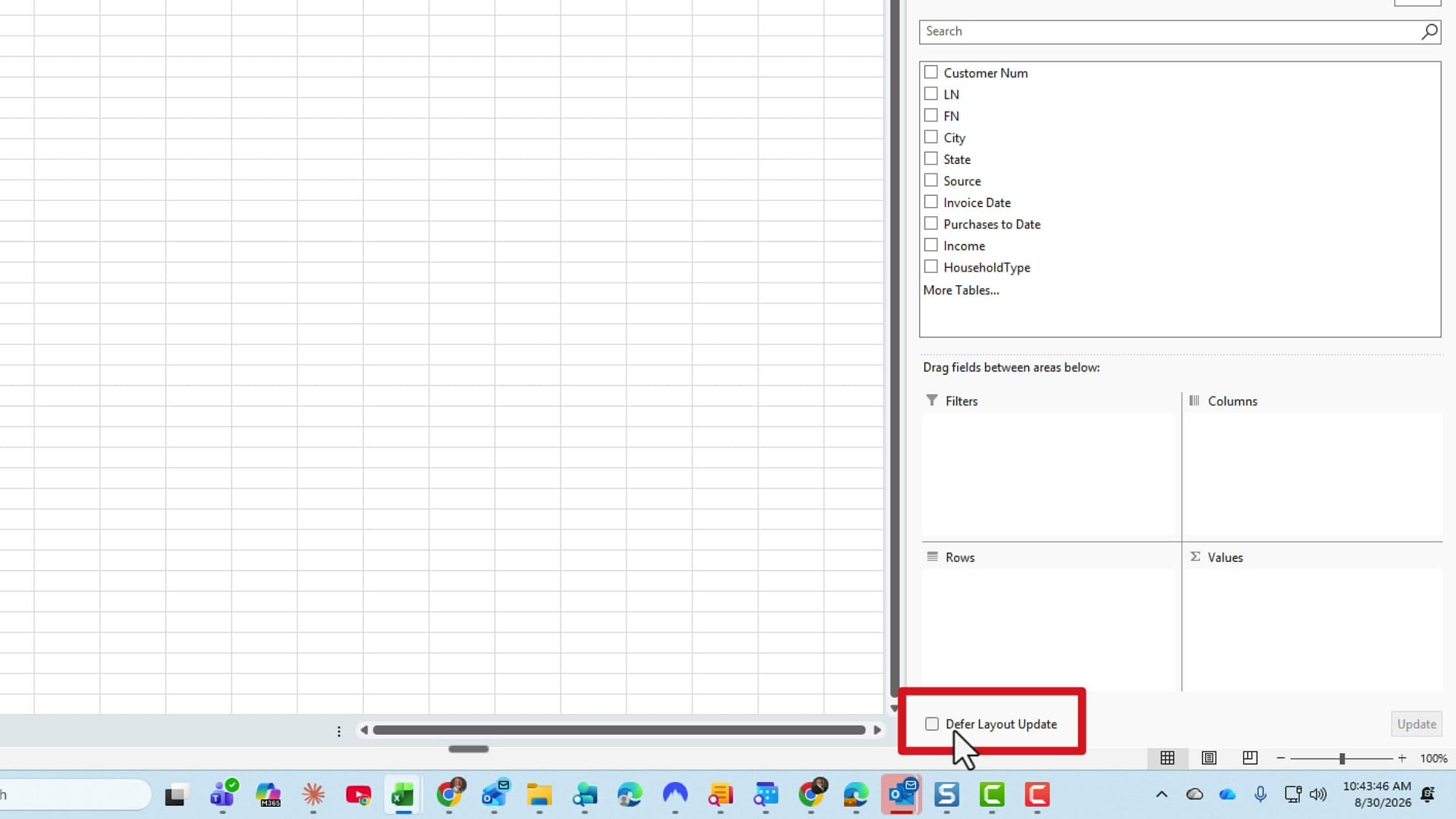
Excel PivotTable from table or range dialog with tbl_customers in the Table/Range box and New Worksheet selected — Insert > PivotTable picks up the table name automatically. New Worksheet is the default.

With a file this size, Excel takes a second to create the PivotTable. When it does, look at the PivotTable Fields pane. Below the field list are the four areas: Filters, Columns, Rows, and Values. And at the very bottom of the pane is the Defer Layout Update checkbox, with a grayed-out Update button next to it.

PivotTable Fields pane with the Filters, Columns, Rows, and Values areas and the Defer Layout Update checkbox highlighted at the bottom — Defer Layout Update sits at the bottom of the PivotTable Fields pane. The Update button stays gray until you turn it on.

The default behavior: updates after every change

I checked State, then City, then Purchases to Date. Excel puts State and City in Rows and Sum of Purchases to Date in Values, and the PivotTable redraws after each checkbox.

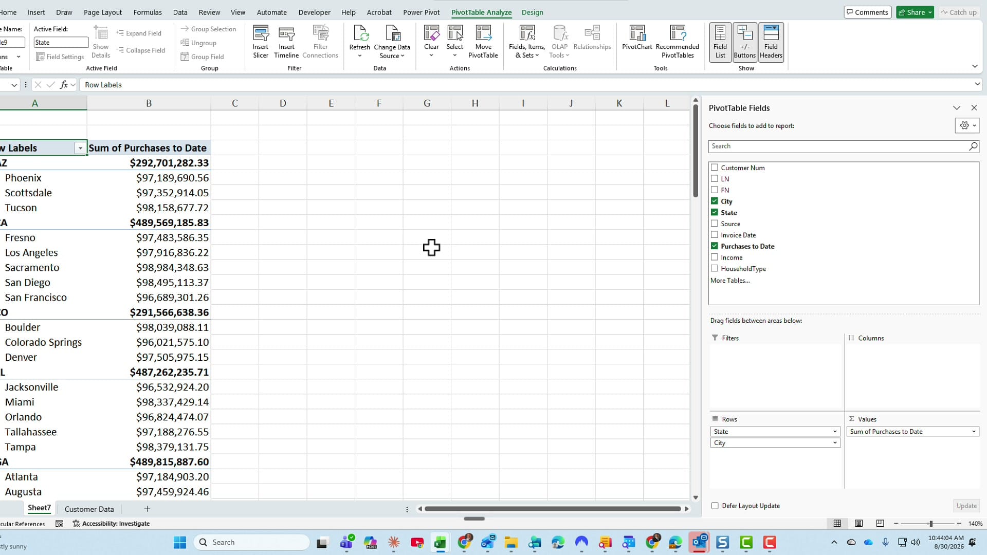
Excel PivotTable showing Sum of Purchases to Date by state and city, with State and City in Rows and Purchases to Date in Values — Without Defer Layout Update, the PivotTable recalculates each time you add or remove a field.

My computer is fast, so the delay here is small. On a slower machine, or with an even bigger data set, waiting after every click adds up fast.

Turn on Defer Layout Update

Check the Defer Layout Update box. The Update button on the right becomes available.

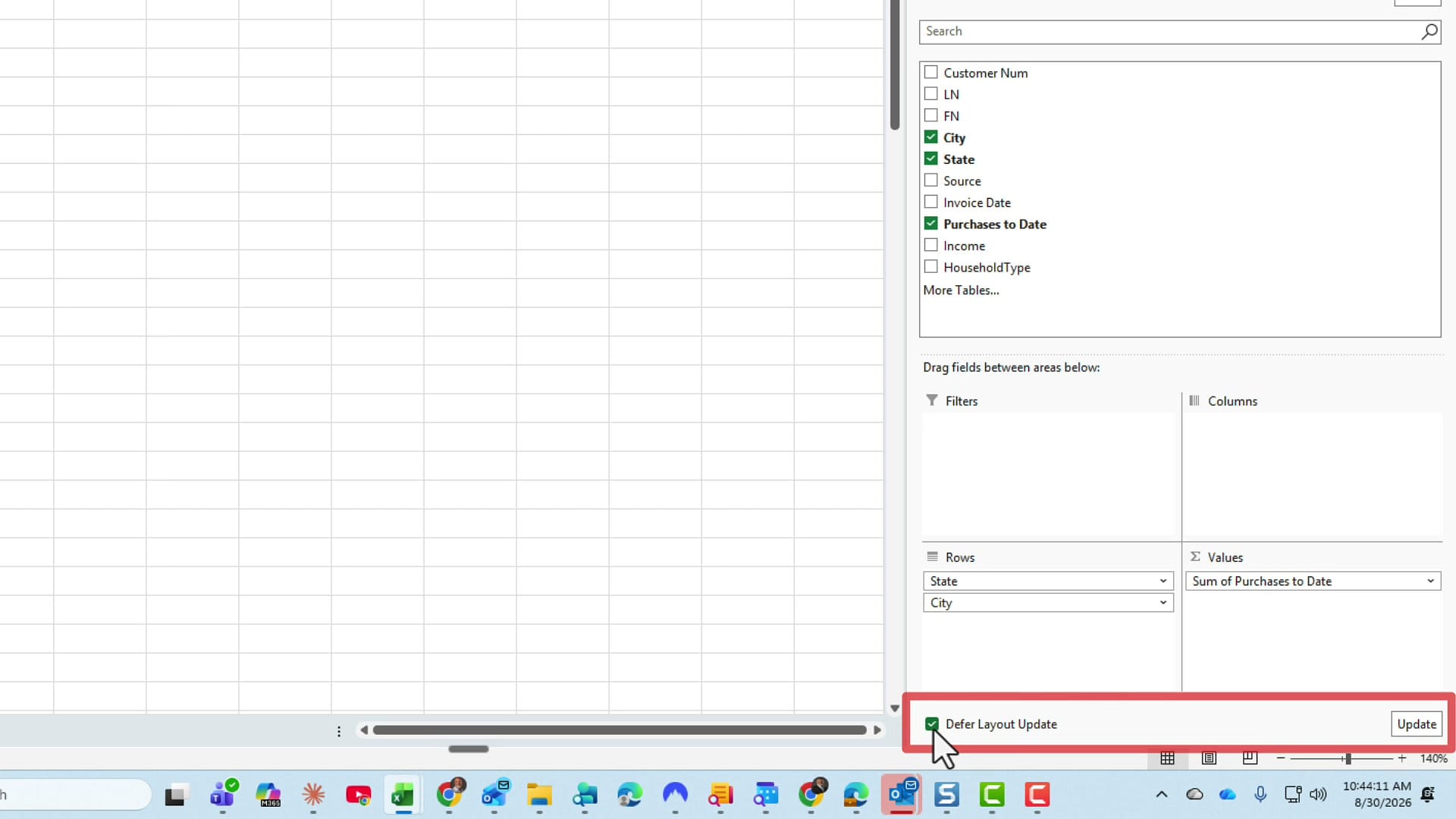
Defer Layout Update checkbox turned on in the PivotTable Fields pane with the Update button now active — Once Defer Layout Update is checked, the Update button is active.

From now on, you can add fields, remove them, and drag them between areas, and nothing happens to the PivotTable until you click Update.

Arrange your fields, then click Update

Here is how I rearranged the layout:

Check HouseholdType and Source. The PivotTable does not change.
Drag HouseholdType into Columns. Still no change.
Drag Source up into Filters.

Now all four areas are in use, but the PivotTable on the sheet still only shows State, City, and Purchases to Date.

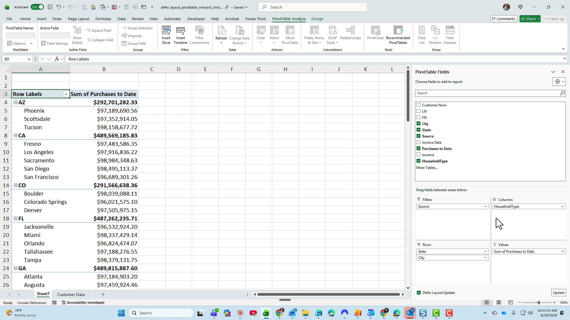
PivotTable Fields pane with Source in Filters, HouseholdType in Columns, State and City in Rows, while the PivotTable still shows only states and cities — All four areas are filled in, but the PivotTable still shows the old layout. Excel is waiting for Update.

Click Update, and everything happens at one time. Source shows up as a report filter above the PivotTable, and each household type becomes its own column.

Excel PivotTable after clicking Update, with a Source report filter and household type columns such as Married, Married with Children, Retired Couple, Roommates, Single, and Single Parent — One click on Update applies every change in a single pass.

Remove and reorder fields

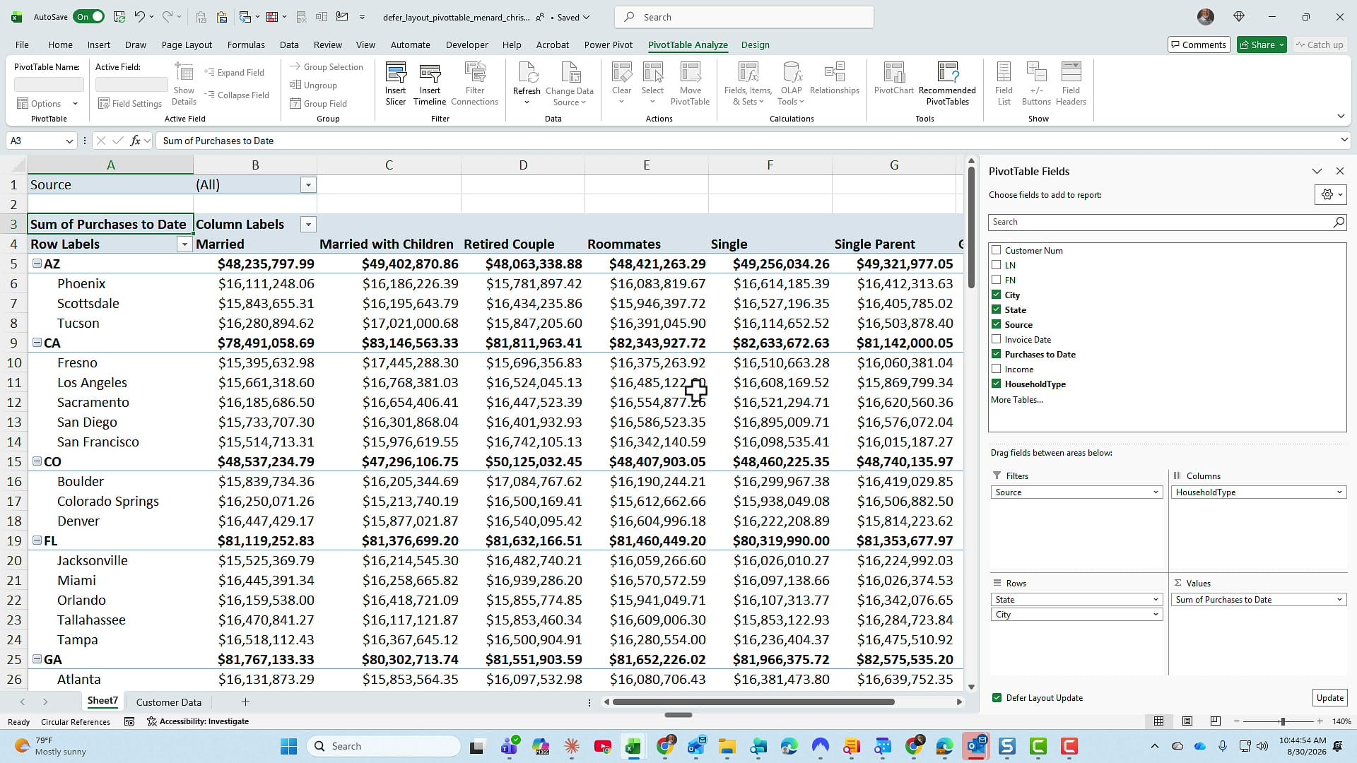
Defer Layout Update stays on until you uncheck it, so you can keep batching changes. For the next pass I wanted to:

Remove Source completely. Click its drop-down in the Filters area and choose Remove Field, or uncheck it in the field list.
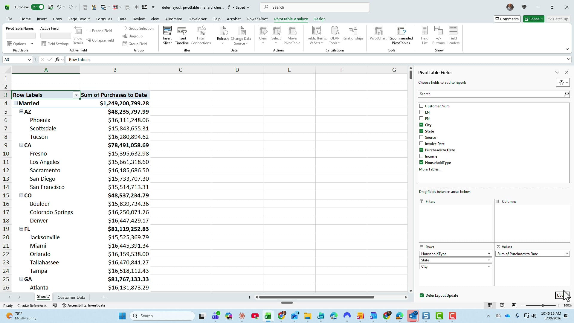
Move HouseholdType from Columns to Rows, above State and City.

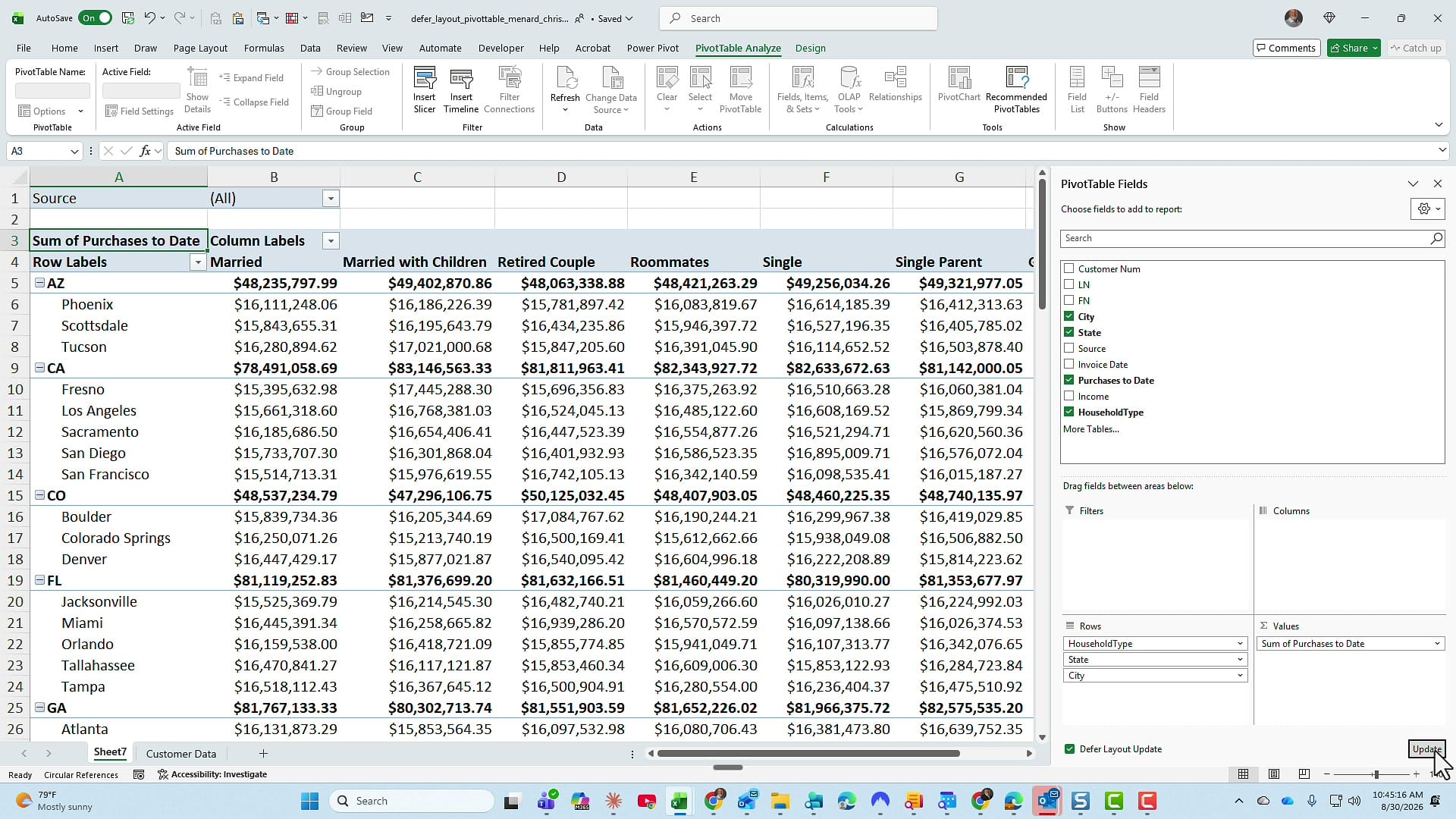
PivotTable Fields pane with HouseholdType dragged to the top of Rows above State and City, Source removed, and the cursor on the Update button — The new layout is ready in the pane: Source removed, HouseholdType at the top of Rows. The PivotTable itself has not changed yet.

Click Update again. The PivotTable now groups by household type first, then state, then city.

Final Excel PivotTable with Married as the top-level row, then states and cities beneath it, showing Sum of Purchases to Date — After the second Update: HouseholdType, then State, then City in the rows.

When to use it

Turn on Defer Layout Update whenever your PivotTable is slow to respond, especially when you plan to make several changes in a row. Build the whole layout, click Update once, and skip all the waiting in between. When you are done, uncheck the box to go back to live updates.

If you are fine-tuning PivotTables often, it is also worth changing the default PivotTable settings so every new PivotTable starts with the layout you want. And if you want the PivotTable to pick up source data changes without clicking Refresh, look at AutoRefresh for PivotTables.