Microsoft Excel

How to Use AutoRefresh for PivotTables in Excel

Chris Menard

05 Aug 2025 — 3 min read

Excel now includes a built-in AutoRefresh option for PivotTables. When enabled, the PivotTable updates automatically any time the underlying data changes — no manual refresh needed.

The Source Data

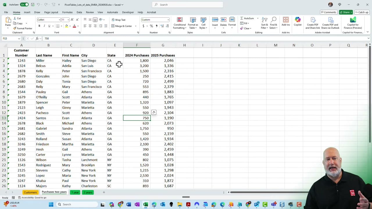
Start with a table of customer data that includes columns for customer number, last name, first name, city, state, and purchase amounts for 2024 and 2025.

Excel spreadsheet showing customer purchase data with columns for Customer Number, Last Name, First Name, City, State, 2024 Purchases, and 2025 Purchases — The source data: a customer table with purchase amounts by year

Creating the PivotTable

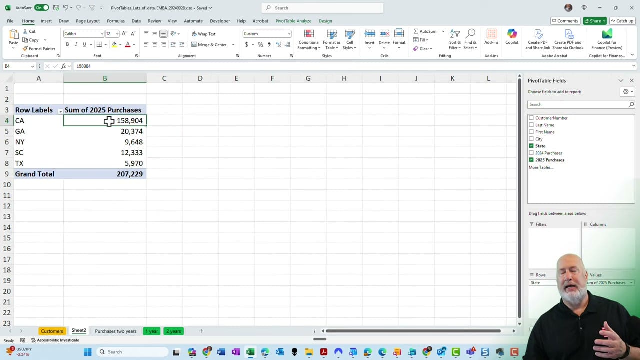
Select the data, go to Insert > PivotTable, and place it on a new worksheet. Drag State into the Rows area and Sum of 2025 Purchases into the Values area. The PivotTable now shows total purchases grouped by state.

PivotTable showing Sum of 2025 Purchases by state with the PivotTable Fields pane open — The PivotTable summarizes 2025 purchases by state — CA leads with 158,904

Testing AutoRefresh

Go back to the source data and change a value — for example, update a purchase amount. Switch to the PivotTable sheet and you'll see the totals update automatically. There's no need to click Refresh or press any shortcut. The PivotTable stays in sync with the data.

YouTube Video

Where to Find the AutoRefresh Toggle

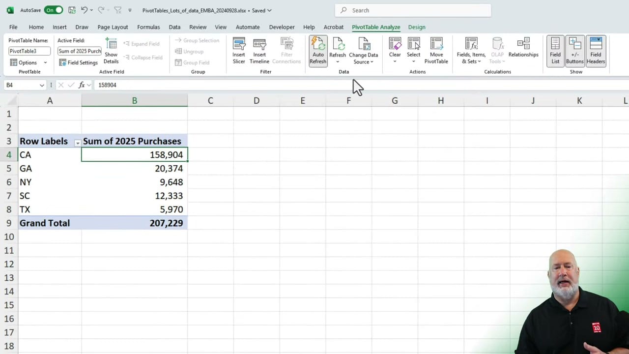
Click inside the PivotTable, then go to the PivotTable Analyze tab on the ribbon. In the Data group, you'll see the Auto Refresh button. It's enabled by default for new PivotTables. If you need to turn it off — for example, when working with very large datasets where constant refreshes slow things down — click the button to toggle it off.

PivotTable Analyze ribbon showing the Auto Refresh button in the Data group — The Auto Refresh button on the PivotTable Analyze tab — toggle it on or off as needed

Excel TRANSLATE Function: Translate Text Directly in Your Spreadsheet

Microsoft has added a built-in TRANSLATE function to Excel that lets you translate text between languages directly in your spreadsheet — no copy-pasting into Google Translate or third-party tools. In this tutorial, Chris Menard demonstrates how to use this powerful new function. YouTube Video How the TRANSLATE Function Works The syntax

Preview: Excel COPILOT() Function and Formula Completion in Action

Live Stream on M365 Copilot Function and Formula Completion in Excel. Registration is NOT required. Just join at noon ET on 03/18/2026

IHG Points vs. Money: How to Save Over 50% on Hotel Rooms Using Excel to Compare

If you're an IHG One Rewards member, you might be leaving serious money on the table by paying cash for hotel rooms. Let me walk you through a real example where I saved over 50% — more than $1,900 — on a four-night stay at one of Washington, DC&

Join Me at the Administrative Professional Conference (APC) 2026 in Nashville for M365 Copilot Essentials

I'll be presenting in-person on M365 Copilot at the APC Conference on September 13-16, 2026, in Nashville, where I’ll show how Copilot works across Excel, Word, PowerPoint, Teams, Outlook, and OneDrive to help administrative professionals work faster and smarter.