Microsoft Excel

How to Find and Remove Extra Spaces in Excel with Conditional Formatting

Chris Menard

16 May 2025 — 3 min read

Extra spaces in Excel data cause real problems — inconsistent sorting, broken lookups, and formulas that return unexpected results. The tricky part is that extra spaces are invisible. Here's how to use conditional formatting with the TRIM function to find them, and then fix them.

The Problem: Hidden Extra Spaces

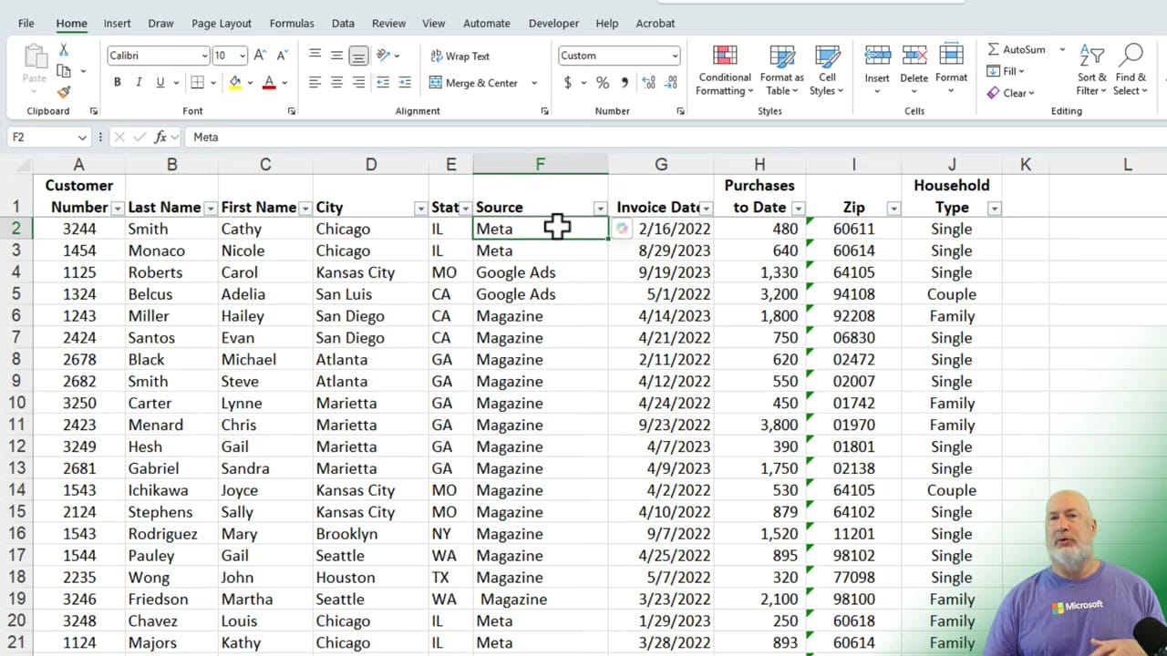
Look at a dataset with a Source column containing values like "Meta," "Google Ads," "Magazine," and "Newspaper." Everything looks fine at first glance, but some cells have leading or trailing spaces that you can't see. This causes problems when sorting — entries that should group together end up separated.

Excel spreadsheet showing customer data with Source column containing Meta, Google Ads, Magazine, and Newspaper entries — The data looks clean, but some Source values have hidden leading or trailing spaces

Using Conditional Formatting to Find Extra Spaces

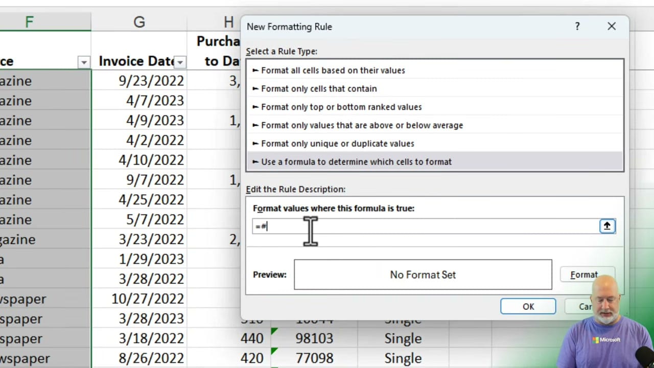
Select the column you want to check. Go to Home > Conditional Formatting > New Rule. Choose "Use a formula to determine which cells to format." Enter the formula:

=F2<>TRIM(F2)

This compares each cell to its TRIM'd version. If they're different, the cell has extra spaces. Set the format to a highlight color (like yellow) and click OK.

New Formatting Rule dialog in Excel with the formula =# entered and Use a formula to determine which cells to format selected — The conditional formatting rule compares each cell to its TRIM'd version to find cells with extra spaces

Seeing the Results

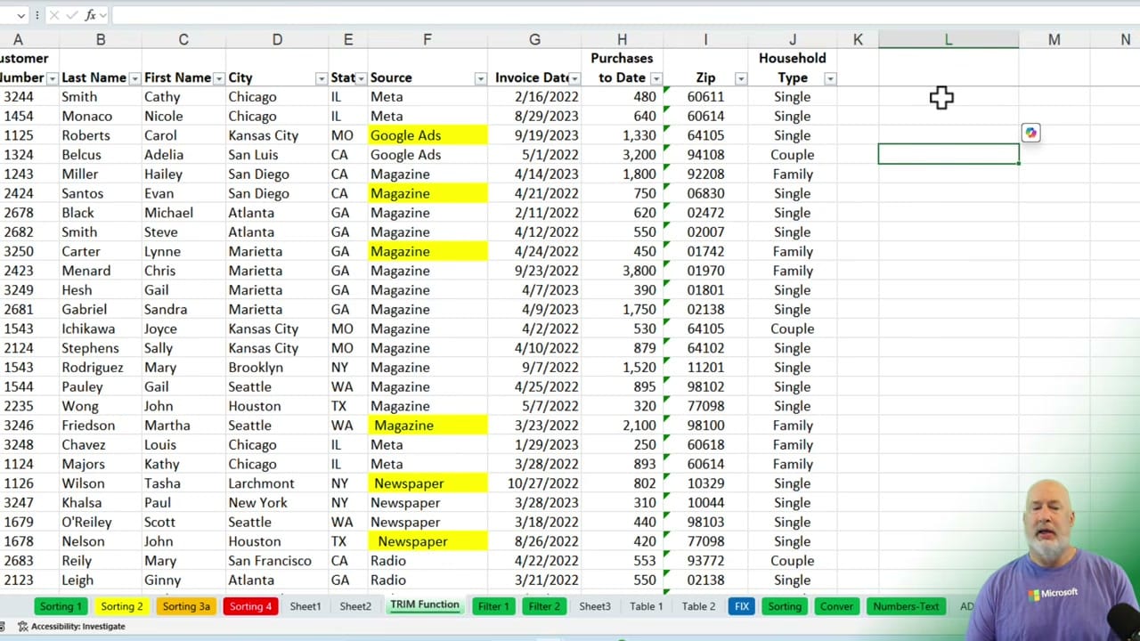
After applying the rule, cells with extra spaces are highlighted immediately. In this example, several "Magazine" and "Newspaper" entries light up — they have leading spaces that weren't visible before.

Excel spreadsheet with conditional formatting applied showing highlighted cells in the Source column where extra spaces were found — The highlighted cells reveal which entries have hidden extra spaces — several Magazine and Newspaper values are affected

Fixing the Data with TRIM

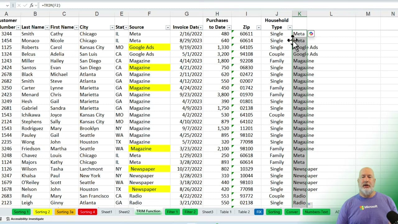
To fix the extra spaces, create a helper column with the formula =TRIM(F2). This returns the cleaned version of each value. Copy the TRIM'd values, paste them back over the original column using Paste Special > Values, and then delete the helper column.

Excel showing a helper column K with TRIM formula results next to the original Source column, with highlighted cells still visible — The TRIM helper column produces clean values — paste these back over the originals to fix the data

After the fix, the conditional formatting highlights should disappear, confirming that all extra spaces have been removed.

Excel TRANSLATE Function: Translate Text Directly in Your Spreadsheet

Microsoft has added a built-in TRANSLATE function to Excel that lets you translate text between languages directly in your spreadsheet — no copy-pasting into Google Translate or third-party tools. In this tutorial, Chris Menard demonstrates how to use this powerful new function. YouTube Video How the TRANSLATE Function Works The syntax

Preview: Excel COPILOT() Function and Formula Completion in Action

Live Stream on M365 Copilot Function and Formula Completion in Excel. Registration is NOT required. Just join at noon ET on 03/18/2026

IHG Points vs. Money: How to Save Over 50% on Hotel Rooms Using Excel to Compare

If you're an IHG One Rewards member, you might be leaving serious money on the table by paying cash for hotel rooms. Let me walk you through a real example where I saved over 50% — more than $1,900 — on a four-night stay at one of Washington, DC&

Join Me at the Administrative Professional Conference (APC) 2026 in Nashville for M365 Copilot Essentials

I'll be presenting in-person on M365 Copilot at the APC Conference on September 13-16, 2026, in Nashville, where I’ll show how Copilot works across Excel, Word, PowerPoint, Teams, Outlook, and OneDrive to help administrative professionals work faster and smarter.