Microsoft Excel

How to Find Duplicates Across Excel Worksheets Using COUNTIF

Chris Menard

13 Mar 2025 — 5 min read

When you have employee data, customer lists, or inventory records spread across multiple worksheets, identifying duplicates between them can be tricky. The COUNTIF function makes this straightforward — and with a few extra steps, you can add visual formatting and custom labels to make the results even clearer.

Understanding COUNTIF

Before jumping into the cross-worksheet approach, here's a quick refresher on how COUNTIF works. The syntax is simple:

=COUNTIF(range, criteria)

It counts how many cells in a range match the specified criteria. In this example, the formula =COUNTIF(H2:H6,G8) counts how many times "atlanta" appears in the city list — and returns 2.

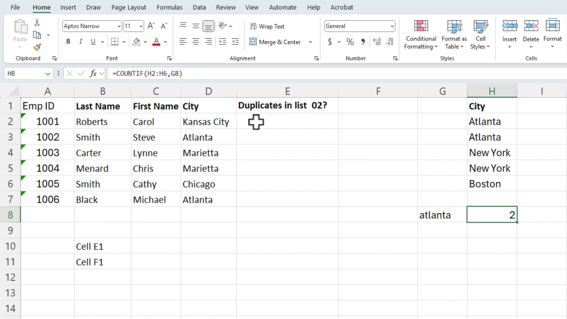
Excel showing =COUNTIF(H2:H6,G8) in cell H8, returning 2 for the search term atlanta against a list of cities including Atlanta, New York, and Boston — =COUNTIF(H2:H6,G8) returns 2 — counting the two Atlanta entries in the city list

Notice that COUNTIF is not case-sensitive — "atlanta" in lowercase still matches "Atlanta" in the list.

Setting Up the Worksheets

For this example, there are two worksheets: List 1 and List 2. Each contains employee records with Emp ID, Last Name, First Name, and City. The goal is to check which Emp IDs from List 1 also appear in List 2.

List 1 contains Emp IDs: 1001, 1002, 1003, 1004, 1005, 1006. List 2 contains: 1001, 1002, 1003, 1005, 1007, 1009. Some overlap, some don't.

Using COUNTIF Across Worksheets

Start by switching to the List 2 worksheet and selecting column A (the Emp ID column). This is the range you'll search against.

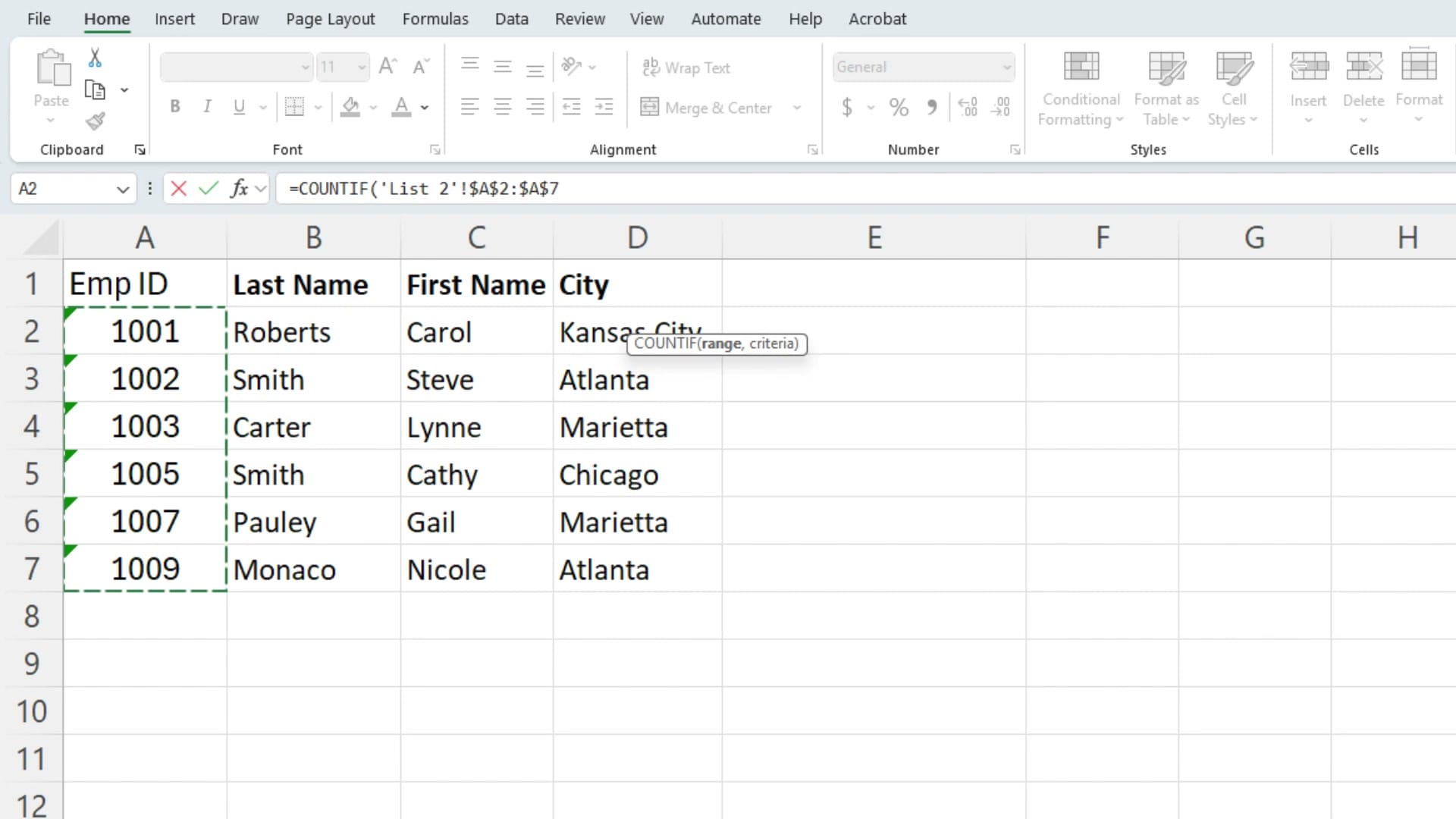
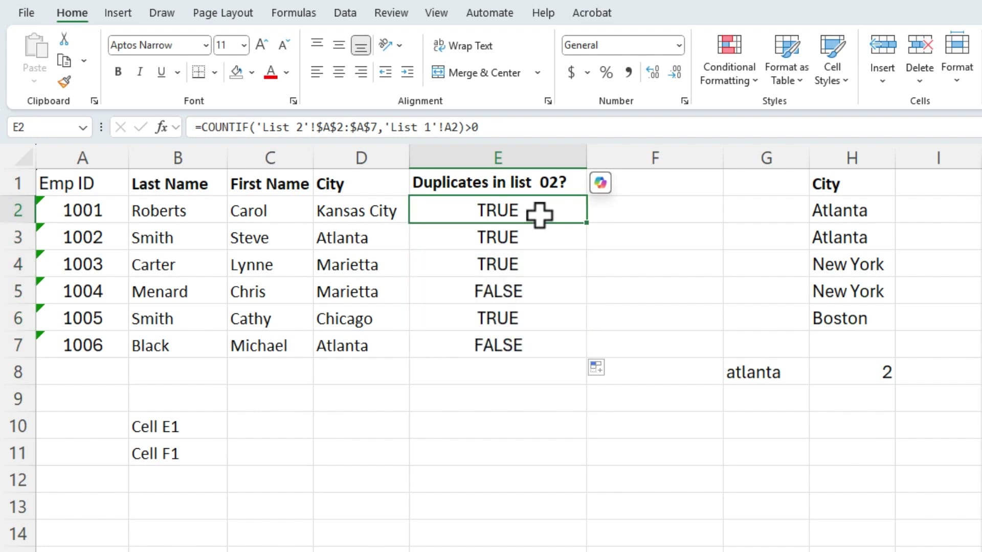
List 2 worksheet showing Emp IDs 1001, 1002, 1003, 1005, 1007, 1009 in column A with dashed selection border, and COUNTIF syntax tooltip visible — On List 2, select the Emp ID range — notice the dashed border indicating the cross-sheet selection

Back on List 1, the formula in cell E2 is:

=COUNTIF('List 2'!$A$2:$A$7,'List 1'!A2)

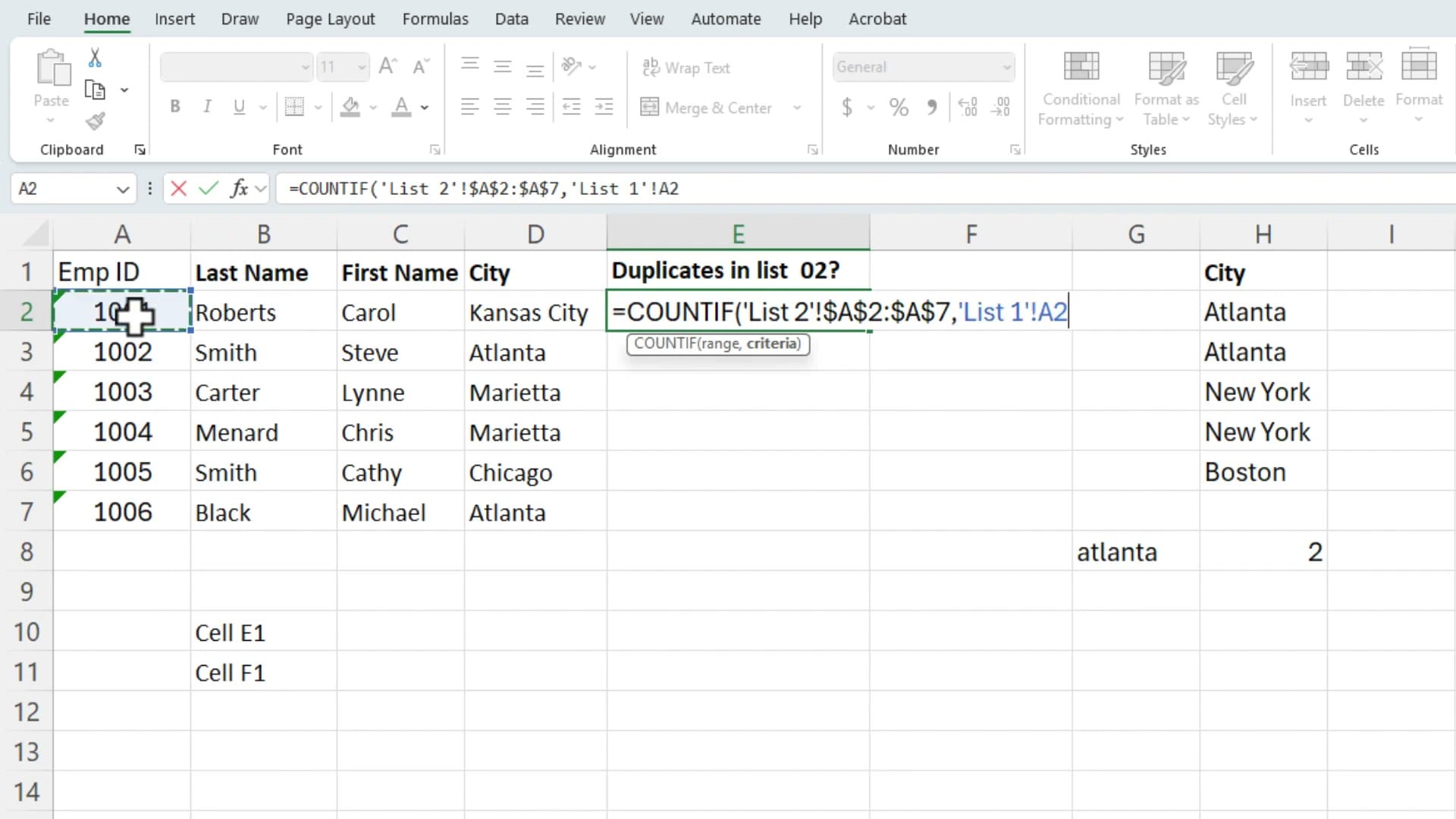
Two critical details in this formula:

Absolute references on the range ($A$2:$A$7) — The dollar signs lock the range so it doesn't shift when you copy the formula down. Without them, the range would move and give incorrect results.
Relative reference on the criteria (A2) — This changes as you copy down, so each row checks its own Emp ID.

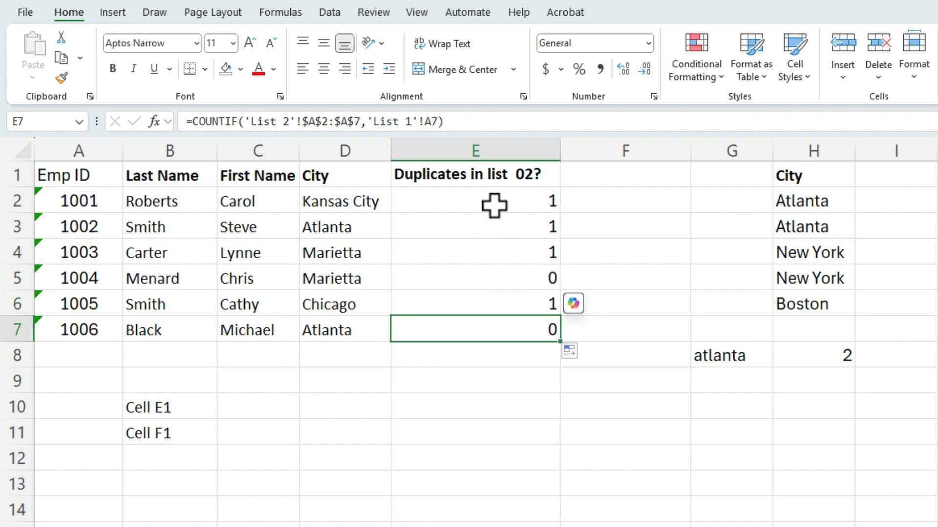
After entering the formula and copying it down through E7, each cell shows either 1 (found in List 2) or 0 (not found):

Excel showing COUNTIF results in column E: 1, 1, 1, 0, 1, 0 for Emp IDs 1001 through 1006, with the formula bar displaying =COUNTIF('List 2'!$A$2:$A$7,'List 1'!A7) — Results: Emp IDs 1001, 1002, 1003, and 1005 return 1 (found in List 2), while 1004 and 1006 return 0 (not found)

Converting Results to TRUE/FALSE

Numbers are fine, but TRUE/FALSE values are often easier to read at a glance. Add >0 to the end of the formula:

=COUNTIF('List 2'!$A$2:$A$7,'List 1'!A2)>0

This converts any count greater than zero to TRUE, and zero to FALSE.

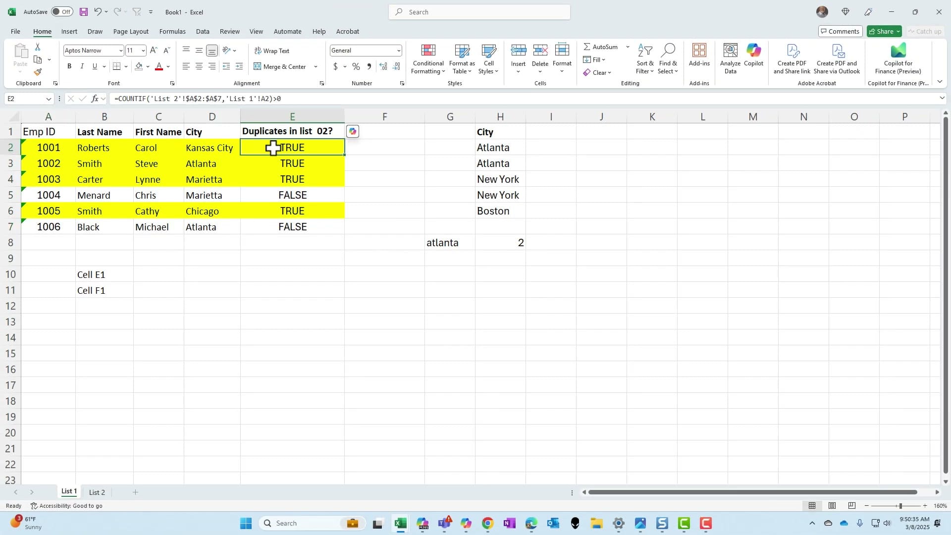
Adding Conditional Formatting

To make duplicates visually obvious, apply conditional formatting that highlights entire rows when column E shows TRUE.

Select the data range (A2:E7)
Go to Home > Conditional Formatting > New Rule
Choose "Use a formula to determine which cells to format"
Enter the formula: =$E2=TRUE
Click Format and choose a fill color (yellow works well)

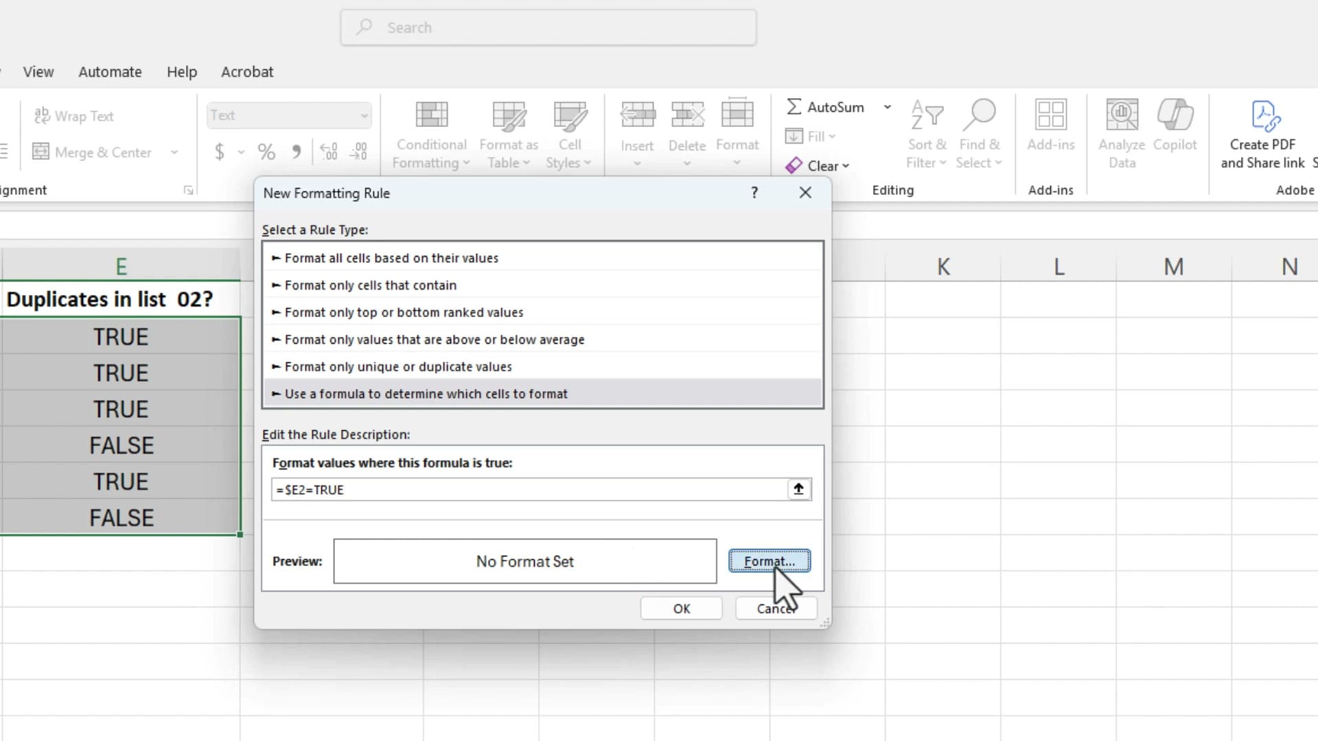
New Formatting Rule dialog in Excel with 'Use a formula to determine which cells to format' selected, showing the formula =$E2=TRUE and the Format button highlighted — The conditional formatting rule uses =$E2=TRUE — the dollar sign on $E locks the column reference so the rule checks column E for every cell in the row

The dollar sign before E ($E2) is important — it locks the column reference to E while allowing the row to change. This way, the formatting checks column E for each row but applies the highlight across all columns.

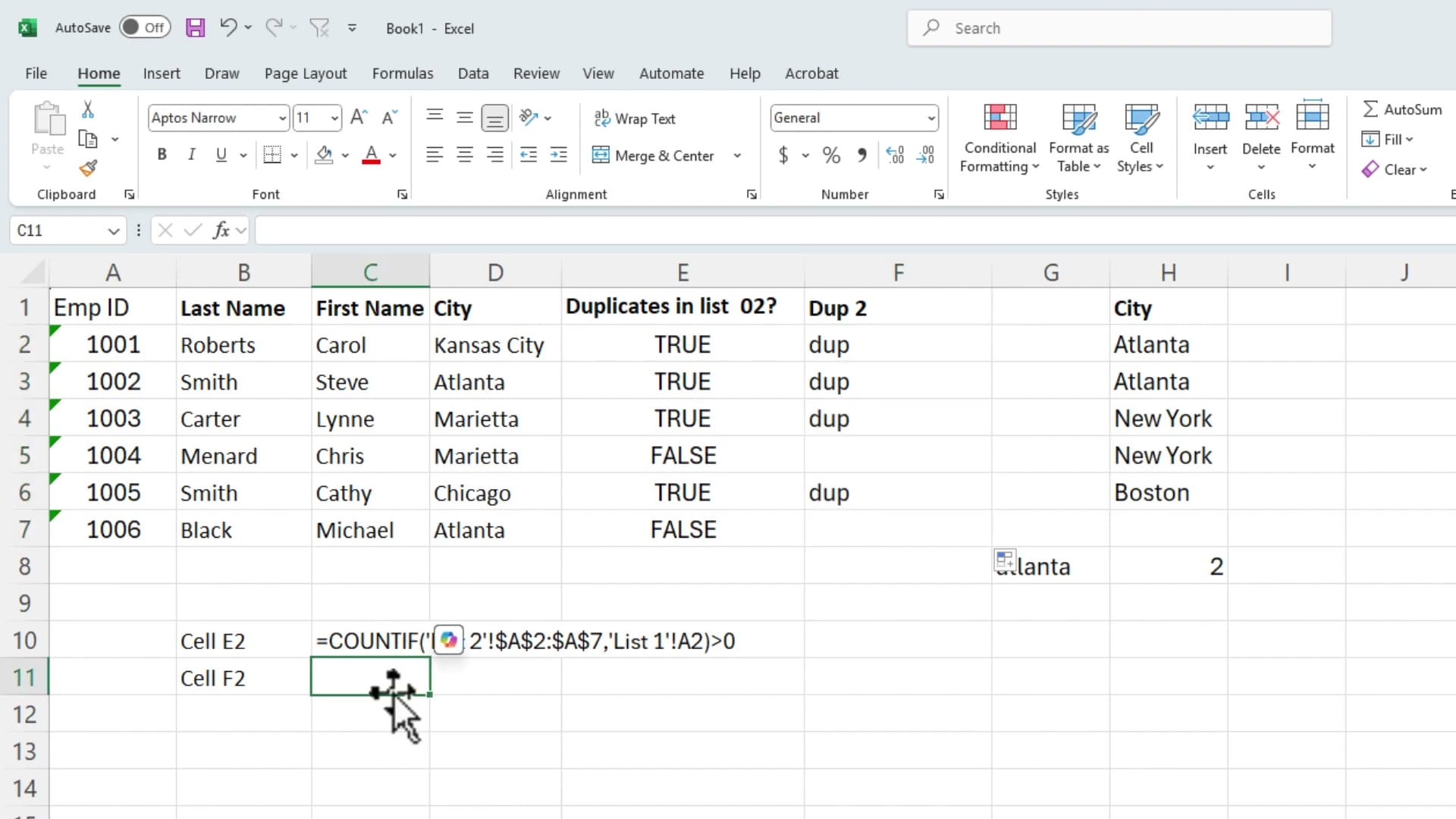
Excel showing rows with TRUE values highlighted in yellow (Emp IDs 1001, 1002, 1003, 1005) while rows with FALSE remain white (Emp IDs 1004, 1006) — Rows with duplicates are now highlighted in yellow — Emp IDs 1004 (Menard) and 1006 (Black) are unique to List 1

Customizing Output with the IF Function

Instead of TRUE/FALSE, you might want a custom label like "dup" for duplicates. Wrap the COUNTIF formula inside an IF function:

=IF(COUNTIF('List 2'!$A$2:$A$7,'List 1'!A2)>0,"dup","")

This returns "dup" when a match is found and leaves the cell blank otherwise. You can also use FORMULATEXT to display the formula in a cell for documentation purposes — just point it at the cell containing the formula:

=FORMULATEXT(E2)

Excel showing column F with 'dup' labels for matching rows (1001, 1002, 1003, 1005) and blank for non-matches, with the COUNTIF formula displayed in cell B10 using FORMULATEXT — The IF function returns "dup" for duplicates and blank for unique entries — cells B10 and B11 use FORMULATEXT to display the underlying formulas

Key Takeaways

COUNTIF across sheets — Use the syntax =COUNTIF('Sheet'!$Range,Criteria) with absolute references on the range
TRUE/FALSE conversion — Append >0 to turn numeric counts into Boolean values
Conditional formatting — Use =$E2=TRUE with a locked column reference to highlight entire rows
Custom labels — Wrap in IF() to display "dup", "match", or any text you prefer
FORMULATEXT — Display the formula from any cell as text for reference or documentation