Excel PivotTable - Summarize data by Month or Day of the week


If you need to find out what day of the week is the most profitable or what day of the week do we receive the most support calls, Excel's PivotTables can handle it. PivotTables will group dates automatically. If you have any date field - invoice dates, order dates, hire dates - Excel will group by year, quarter, and month for you. No formula's needed.
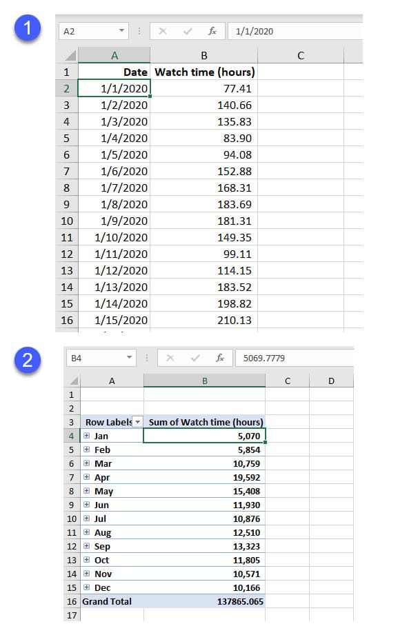
Image 1 is Excel starting on January 1. The data went to December 31. In Image 2, is Excel's PivotTable automatically grouping the months in column A.
If you want to group by day of the week, we can use the **TEXT** function in Excel and group by the day of the week. In this example, I use PivotTable and the Text function to find out what day of the week do my YouTube videos get the most watch time in hours.
YouTube video
Excel PivotTable - Summarize data by Month or Day of the week
TEXT Function in Excel
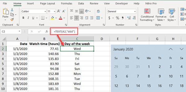
The TEXT function returns a number or date in a given number format, as text. I use the text function to get the date formatted as a three-letter date in the video. Example: 1/1/2020, which is a Wednesday, I showed as Wed.
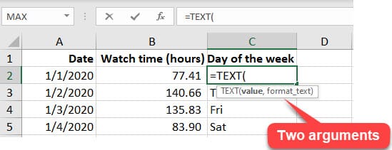
TEXT Function Arguments
The text function has two arguments. Both arguments are required.
**=TEXT(Value,Format Text)**
- value - The number to convert. - format\_text - The number format to use.
TEXT Function Examples
Below are some TEXT function examples for dates. Month is the letter "M", day is the letter "D", and year is the letter "Y".
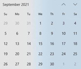
We are going to use the month of September 2021 in our example
The letter D
| **Date** | **d** | **dd** | **ddd** | **dddd** | | --- | --- | --- | --- | --- | | 9/1/2021 | =Text(A2,"d") would return **1** | =Text(A2,"dd") would return **01** | =Text(A2,"ddd") would return **Wed** | =Text(A2,"dddd") would return **Wednesday** |
The letter M
| **Date** | **d** | **dd** | **ddd** | **dddd** | | — | — | — | — | — | | 9/1/2021 | =Text(A2,"m") would return **1** | =Text(A2,"mm") would return **01** | =Text(A2,"mmm") would return **Sep** | =Text(A2,"mmmm") would return **September** |
Create a PivotTable
A PivotTable is a powerful tool to calculate, summarize, and analyze data that lets you see comparisons, patterns, and trends in your data.
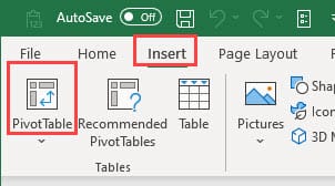
1. Click inside your data. Make sure your data doesn't have any blank rows or columns and only a single header row. 2. Click the **Insert** tab and select **PivotTable.**
**
**
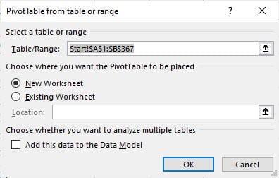
3. Your Table/Range will be selected. Make sure it is correct. You can make the PivotTable in a new worksheet or existing worksheet. To create the PivotTable on a new worksheet click **OK.**
**
**
Build your PivotTable
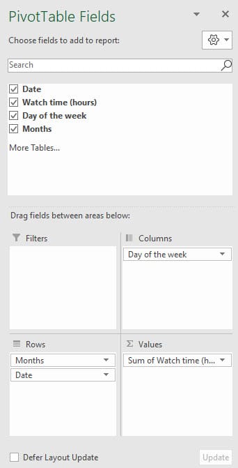
The PivotTable Fields pane appears on the left. There are four areas:
- Filters - Columns - Rows - Values
Add fields to the PivotTable
1. Your header rows from your data are called PivotTable fields. 2. Drag and drop the fields to create a PivotTable. You can check the fields also to create a PivotTable. You can move fields by dragging to another area.