Excel Charts - three methods for filtering Chart Data

Posted on:  02/26/2021

Filtering data in Excel charts is easy to do. The method you use should be based on the amount of data you have. In this video, I show three methods of filtering chart data. Method 1 is using Chart Filters. This is the easiest method. Method 2 is using Filters and creating a chart. Method 3 is using a Table and Filters. Methods 2 and 3 work great with large data sets. Method 1 is great for a small set of data. I also show Transpose data and how to keep a chart from moving or disappearing when you filter your data.

 

YouTube Video on filtering charts

Method 1 - Using Chart Filters

Steps to use Chart Filters

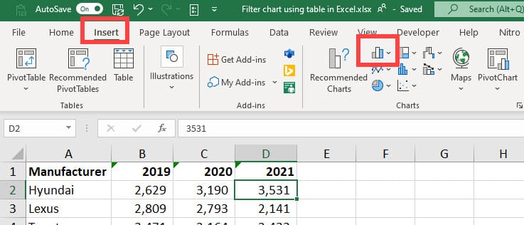
1. Select your data to chart.
2. Click the Insert tab, and select the chart you want to use. I used a column chart (2d) in the video.
   
    
3. After the chart is added to the worksheet, click Chart Filters.
   
    
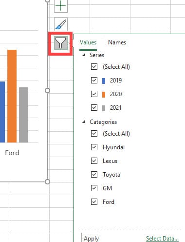
4. Uncheck the data you do not want to see in the chart.
5. Click Apply.

Method 2 - Filter the data and let the chart change

Filtering your data is a great way to handle chart filters with a lot of data. When you filter the data, the chart will change.  One issue we're going to have to address is making sure the chart stays on the screen. When you filter, you get hidden rows, and occasionally, the chart will be in those hidden rows.

Steps to use Data Filters to change the chart

1. Click inside your data range.
2. Click the Data tab, and turn on Filters by clicking Filters. Your header row will have drop down arrows.
3. Create a chart by going to Insert tab and selecting a columns chart.
4. Now filter your data using the drop down arrows in the data. Don't use the Chart Filters.

Note: to keep your chart from moving or resizing, see the next section.

Keep Chart from moving or resizing

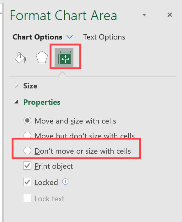
When you filter your data, your chart could get hidden with the rows that get hidden. To keep your chart always visible when filtering data, turn on Chart Properties - Don't size or move with cells.

1. Create your chart.
2. Righ-click in the chart and select Format Chart Area...
3. Select Size and Properties
4. Expand properties.
5. Select Don't move or size with cells.

Method 3 - Filter the data using a Table and let the chart change

Using a Table is similar to Method 2, using a range, but you have advantages with tables over ranges. When you change your range to a Table and add data, the chart automatically updates. With a range, you will have to change the data source.

 

To create a table

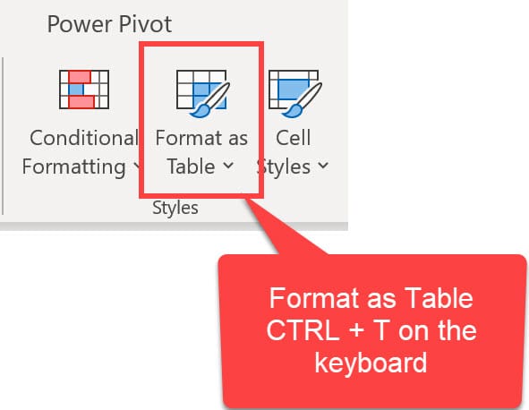
1. Click inside your data and use CTRL + T or use the Home tab, Format as Table

 

Categories

• Blog » Microsoft » Microsoft Excel » Intermediate