Microsoft Excel

How to Change Default PivotTable Settings in Excel to Save Time

Chris Menard

16 Sep 2025 — 4 min read

Every time you create a PivotTable in Excel, you get the same default layout: compact form, subtotals at the top, grand totals on, and columns that auto-resize. If you always change these settings manually, you're wasting time. Excel lets you change the default PivotTable layout so every new PivotTable starts the way you want.

This feature works in Microsoft 365, Excel 2021, and Excel 2019. Here's how to set it up using two different methods.

The Default PivotTable Layout Problem

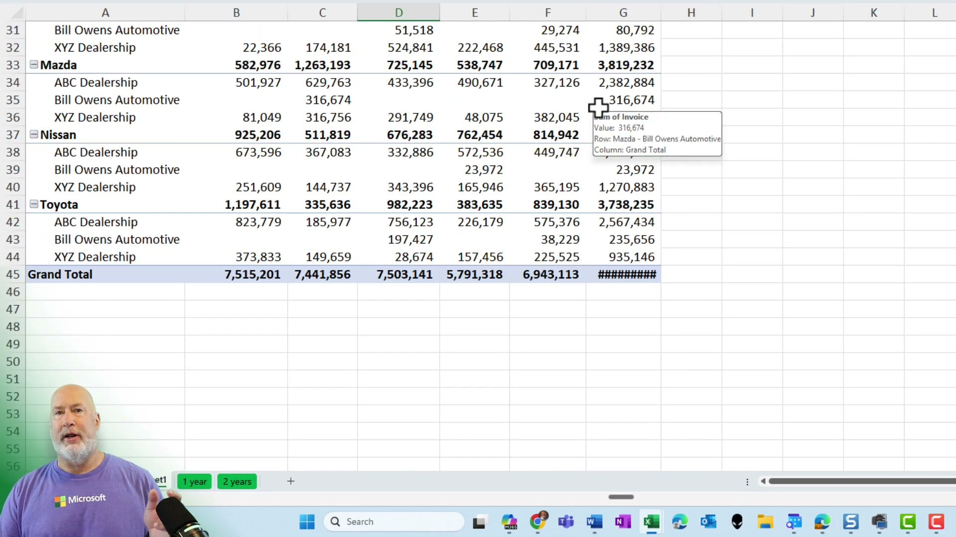
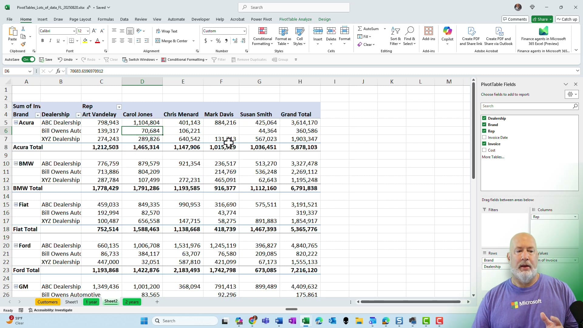
When you create a PivotTable from your data, Excel uses compact layout by default. In compact form, row labels are stacked in a single column with subtotals at the top of each group. For many users, this layout makes the data harder to read — especially when you have multiple row fields like Brand, Dealership, and Rep.

Excel PivotTable in default compact layout showing car dealership invoice data with subtotals at top of each group — The default compact layout stacks row labels in one column with subtotals at the top

Method 1: Edit Default Layout from an Existing PivotTable

If you already have a PivotTable open, go to the PivotTable Analyze tab (or Analyze in some versions), click Options, then select Edit Default Layout. This opens the Edit Default Layout dialog, where you can change four settings:

Subtotals — Move from "Top of Group" to "Bottom of Group" (or turn them off entirely)
Grand Totals — Choose whether to show them for rows, columns, both, or neither
Report Layout — Switch from Compact Form to Show in Tabular Form
Blank Rows — Check "Insert Blank Line after Each Item" for better readability

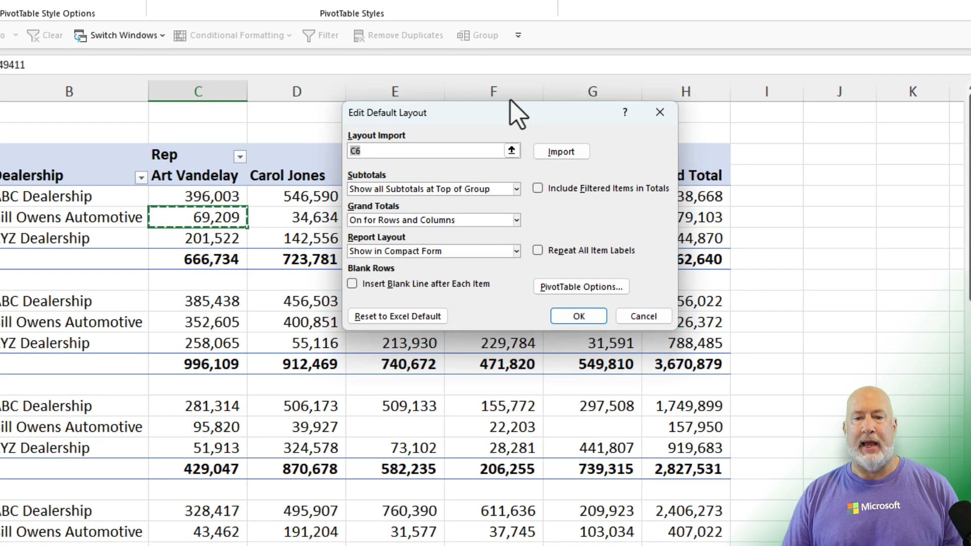
Edit Default Layout dialog in Excel showing options for Subtotals, Grand Totals, Report Layout set to Show in Compact Form, and Blank Rows — The Edit Default Layout dialog lets you change subtotals, grand totals, report layout, and blank rows

You can also click Import to pull settings from an existing PivotTable. If you've already formatted a PivotTable the way you like, select its cell reference and Excel will copy those layout settings as your new defaults.

Method 2: Change Defaults Before Creating a PivotTable

You don't need an existing PivotTable to change defaults. Go to File → Options → Data, then click Edit Default Layout under the Data options. The same dialog appears, and you can configure your preferred settings before creating any PivotTable.

Turning Off AutoFit Column Widths

One more setting worth changing: by default, Excel auto-resizes column widths every time you modify a PivotTable. This can be annoying if you've manually set your column widths. In the Edit Default Layout dialog, click PivotTable Options and uncheck Autofit column widths on update.

Testing Your New Defaults

After changing the defaults, create a new PivotTable to verify. Your new table should automatically use tabular layout with subtotals at the bottom, blank rows between groups, and your preferred grand total settings — no manual reformatting needed.

After changing defaults, new PivotTables automatically use tabular layout with your preferred settings

Key Takeaways

Default settings apply to all new PivotTables — existing ones keep their current formatting
Two methods: from an existing PivotTable (PivotTable Analyze → Options → Edit Default Layout) or from File → Options → Data
The Import button lets you copy settings from a PivotTable you've already formatted
Don't forget to disable AutoFit column widths if you prefer manual control
These settings are per-installation, not per-workbook — they persist across all your Excel files