How to Use GROUPBY with HSTACK for Non-Adjacent Columns in Excel

Excel's GROUPBY function is a formula-based alternative to PivotTables that updates automatically and offers more aggregation options — including MEDIAN, MODE, and custom LAMBDA functions. When you need to group by columns that aren't next to each other, HSTACK lets you combine non-adjacent columns into a single range that GROUPBY can use.

The Source Data

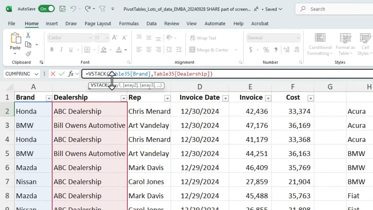
The example uses a car dealership invoice table with columns for Brand, Dealership, Rep, Invoice Date, Invoice Amount, and Cost. The goal is to aggregate invoice totals by Brand and Dealership, then later by Brand and Rep — where Brand and Rep aren't adjacent columns.

Setting Up GROUPBY for Adjacent Columns

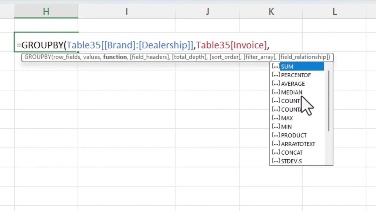
The basic GROUPBY syntax is =GROUPBY(row_fields, values, function). For adjacent columns like Brand and Dealership, you can reference them as a single range:

=GROUPBY(Table35[[Brand]:[Dealership]], Table35[Invoice], SUM)

This group's invoice totals by Brand and Dealership. The function parameter offers many options beyond SUM — you can choose AVERAGE, MEDIAN, COUNT, MAX, MIN, PERCENTOF, and more. Unlike PivotTables, GROUPBY gives you access to aggregation functions that PivotTables don't support natively.

GROUPBY results update automatically when you add or change data in the source table. There's no need to refresh like you would with a PivotTable.

Using HSTACK for Non-Adjacent Columns

What if you want to group by Brand (column A) and Rep (column C)? These columns aren't next to each other, so you can't reference them as a single range. The solution is HSTACK, which horizontally stacks multiple ranges into one:

=GROUPBY(HSTACK(Table35[Brand], Table35[Rep]), Table35[Invoice], SUM)

HSTACK combines the Brand and Rep columns side by side. GROUPBY then treats this combined range as its row_fields parameter, giving you invoice totals grouped by Brand and Rep.

Key Advantages Over PivotTables

• Automatic updates — No manual refresh needed when source data changes
• More aggregation functions — Access MEDIAN, MODE, PERCENTOF, and custom LAMBDA functions
• Formula flexibility — Combine with other dynamic array functions like UNIQUE, SORT, and FILTER
• Non-adjacent grouping — HSTACK lets you group by any columns, regardless of position

Related guides

Easily Combine Ranges with VSTACK and HSTACK in Excel: Chris Menard Training

VSTACK and HSTACK are two great functions in Excel. We will use them to combine ranges.

Menard on MicrosoftChris Menard

Master UNIQUE, CHOOSECOLS, COUNTA & SORT in Excel — Clean Data Fast

Learn how to extract, sort, and count distinct values in Excel using UNIQUE, CHOOSECOLS, COUNTA and SORT. Practical examples, non-adjacent column fixes, and a bonus conditional-formatting tip.

Menard on MicrosoftChris Menard

Excel - Combine the SORT, UNIQUE, and COUNT functions: Chris Menard Training

Excel has dynamic array functions. Two of the dynamic array function are SORT and UNIQUE. I will combine SORT and UNIQUE and also combine them with COUNT and the COUNTA functions. This came from a user that asked how many unique zip codes were in a spreadsheet.

Menard on MicrosoftChris Menard

Want to learn more? Visit courses.chrismenardtraining.com for online training courses.