How to Fix Commas in Data Using Excel Power Query


When your Excel data has multiple values crammed into a single cell — like office locations separated by commas — sorting and filtering become impossible. Power Query can split those values into separate rows, giving you clean, usable data.
The Problem: Comma-Separated Values in One Cell
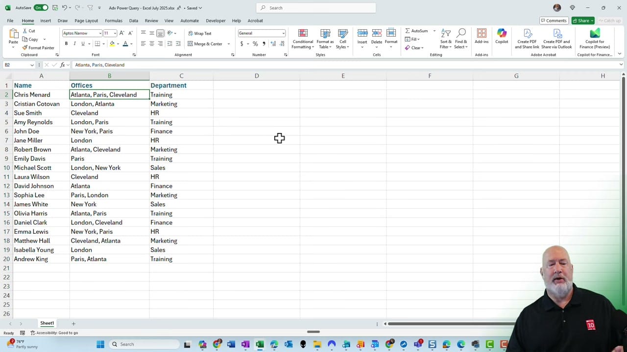
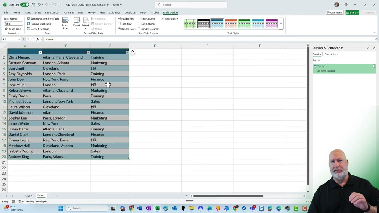
Consider a table with employee names, office locations, and departments. Some employees work from multiple offices, and those offices are listed in a single cell separated by commas (e.g., "Atlanta, Paris, Cleveland"). You can't properly filter or sort by individual office when multiple values share a cell.
Loading the Data into Power Query
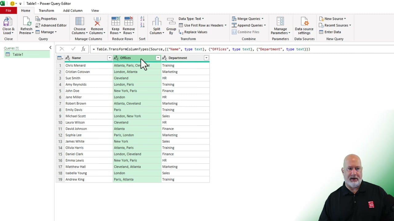
First, format the data as a table if it isn't already. Then go to the Data tab and click From Table/Range. This opens the Power Query Editor with the table loaded.
Splitting the Commas into Separate Rows
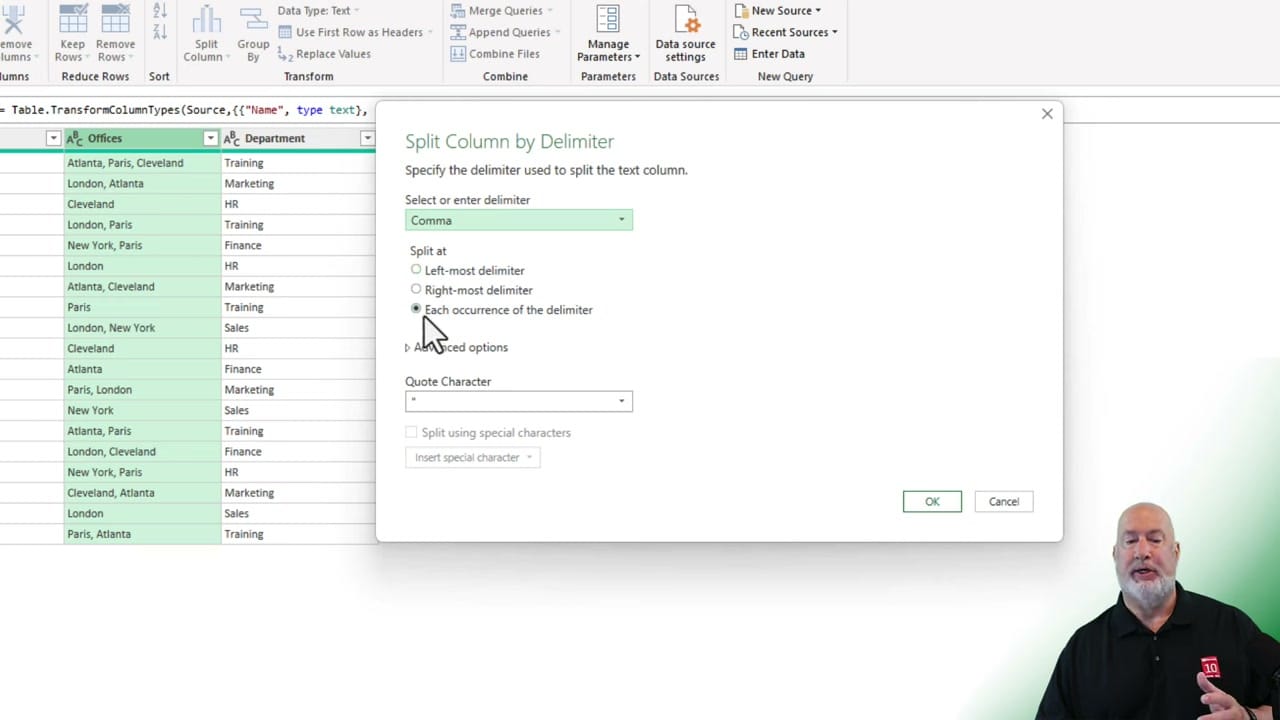
Select the Offices column, then go to Split Column > By Delimiter. Choose Comma as the delimiter. Under "Split at," select Each occurrence of the delimiter. Then expand Advanced options and choose Split into Rows (not columns). Click OK.
The Result: Clean, Individual Rows
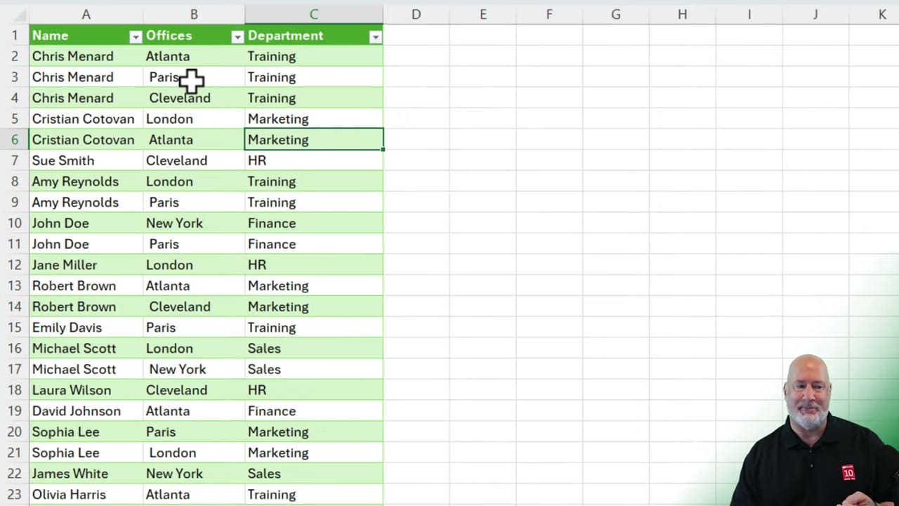
Each comma-separated office now has its own row. An employee with three offices now appears in three rows — one per office. This makes sorting, filtering, and PivotTable analysis straightforward.
Fixing Leading Spaces
After splitting, some values may have a leading space (e.g., " Paris" instead of "Paris"). In the Power Query Editor, right-click the Offices column and select Transform > Trim. This removes any extra spaces from the beginning and end of each value.
Refreshing the Data
When the source data changes — like adding a new employee or updating office assignments — right-click the output table and choose Refresh. Power Query re-runs the transformation automatically.
Related Excel Tutorials