Microsoft Excel

How to Add Filter by Selection to Excel's Quick Access Toolbar

Chris Menard

24 Nov 2025 — 3 min read

Excel's Filter by Selection feature lets you click a cell and instantly filter the entire column to show only matching values — no dropdown menus needed. The catch is that it's hidden by default. Here's how to add it to your Quick Access Toolbar for one-click filtering.

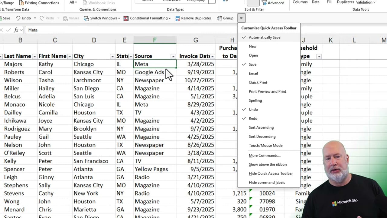
The Quick Access Toolbar (QAT) sits above the ribbon and gives you one-click access to your most-used commands. To customize it, click the small dropdown arrow at the right end of the toolbar and select More Commands.

Excel Quick Access Toolbar dropdown menu showing options like Save, Email, Quick Print, and More Commands at the bottom — Click the QAT dropdown and select "More Commands" to open the customization dialog.

Adding Filter by Selection

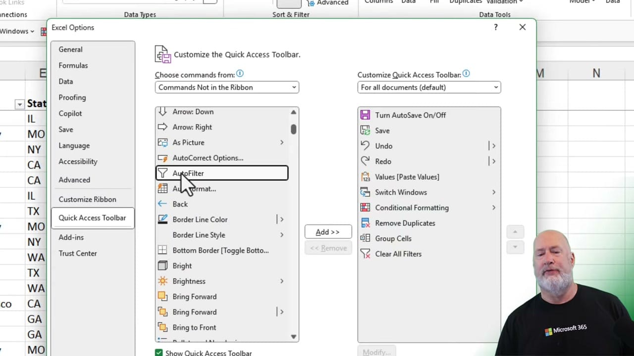
In the Excel Options dialog, select Quick Access Toolbar from the left sidebar. Change the "Choose commands from" dropdown to Commands Not in the Ribbon. Scroll down to find AutoFilter — this is the Filter by Selection command. Click Add to move it to your toolbar. While you're there, also add Clear All Filters so you can quickly remove filters after applying them.

Excel Options dialog showing Quick Access Toolbar customization with AutoFilter selected in the Commands Not in the Ribbon list, and Clear All Filters already added to the toolbar — Find AutoFilter under "Commands Not in the Ribbon" and add it alongside Clear All Filters.

Using Filter by Selection

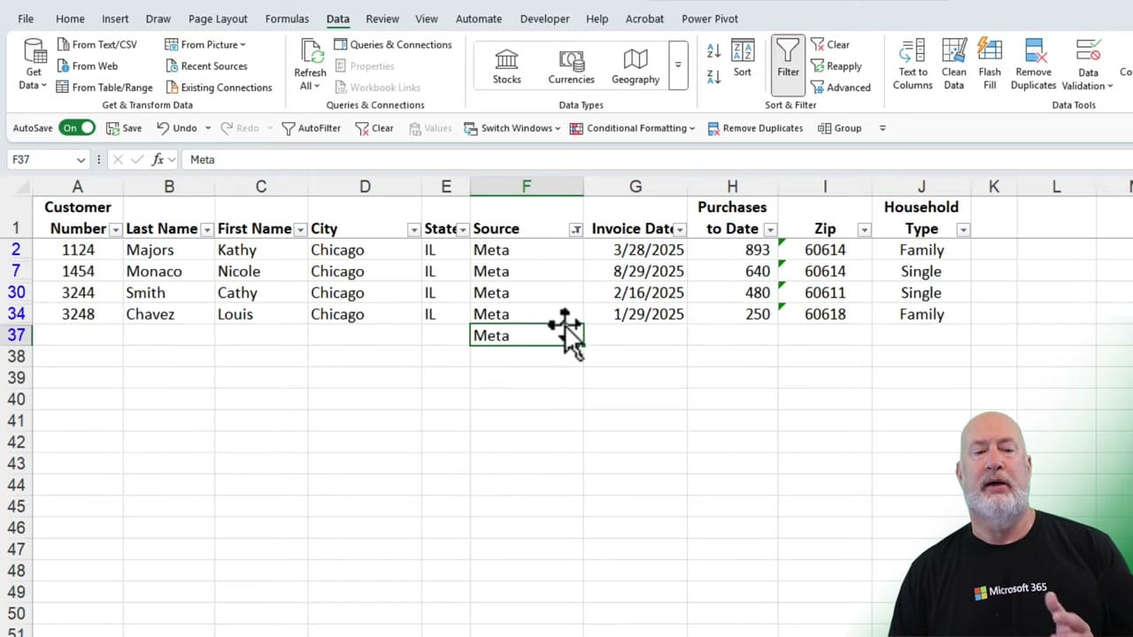
Once added, using it is simple: click any cell containing the value you want to filter by, then click the Filter by Selection button on your QAT. Excel instantly filters the column to show only rows matching that value. For example, clicking a cell containing "Meta" and pressing the button shows only the four Meta entries.

Excel spreadsheet filtered to show only rows where Source column equals Meta, displaying 4 matching records out of the full dataset — One click on Filter by Selection filters the entire dataset to show only "Meta" entries.

Filter by Selection vs. Right-Click Filter

You can also filter by right-clicking a cell and choosing Filter > Filter by Selected Cell's Value. But this takes two clicks through a context menu. The QAT button does it in one click — much faster when you're working with large datasets and need to filter repeatedly.

This works with text, numbers, and dates. You can apply multiple filters across different columns, and use the Clear All Filters button to reset everything at once.