How to Use the Future Value function Correctly in Excel (Monthly Compounding Fix)

If you model investments in Excel, the future value function is one of the most useful tools you have. The problem is a small but common mistake: dividing an annual return by 12 to get the monthly rate. That shortcut breaks the math when compounding is involved, leading to a subtly incorrect future value.

The common mistake with the future value function

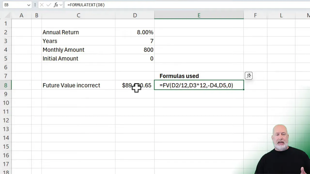
The typical approach looks like this: you have an 8 percent annual return, you want monthly periods, so you enter 8%/12 for the rate and 7*12 for the periods. You then add your monthly contribution and call it done. In Excel, that often becomes a formula like:

=FV(8%/12, 7*12, -800, 0, 0)

That formula seems logical, but it assumes the annual rate simply splits evenly into monthly pieces without compounding. In reality, an annual return of 8 percent compounds throughout the year, so the true monthly return is slightly less than 8%/12. Over several years, that small difference compounds and changes the final value.

Why does annual divided by 12 fails

When returns compound, the correct relationship between an annual nominal rate and the equivalent monthly rate r_m is:

(1 + annual_rate) = (1 + r_m)^(12)

Solving for the monthly rate:

r_m = (1 + annual_rate)^(1/12) - 1

So instead of using 8%/12, compute the monthly rate as (1+8%)^(1/12)-1 and feed that into the future value function. That small adjustment makes Excel produce a value that matches trusted financial calculators and real-world compounding.

Quick visual comparison

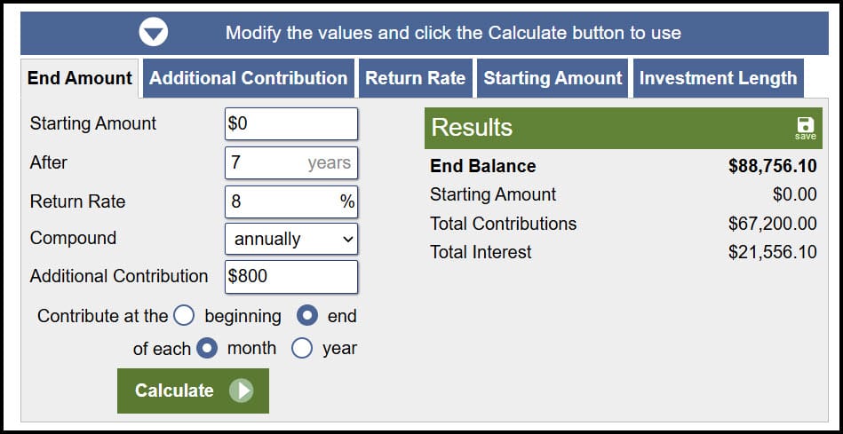
I validated this against an online investment calculator that compounds annually and allows monthly contributions. With zero starting balance, $800 monthly contributions, 7 years, and 8% annual return, the calculator gave a different result than the naive Excel formula. The corrected monthly-rate approach produced a perfect match.

Correcting the future value function in Excel

Replace the naive 8%/12 with the compounded monthly rate. Using the literal approach, the corrected Excel formula looks like this:

=FV((1+8%)^(1/12)-1, 7*12, -800, 0, 0)

Or better, calculate the monthly rate in its own cell (for clarity and reuse), then reference that cell inside FV. For example:

E2 = (1 + D2)^(1/12) - 1   // where D2 contains the annual rate (8%)
F2 = FV(E2, 7*12, -800, 0, 0)
  

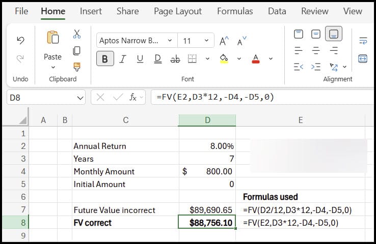
With that change, the future value aligns exactly with the investment calculator. To convince yourself further, test with a $1 principal: after 12 months, the compounded monthly approach yields exactly 1.08, while the naive 8%/12 approach does not.

Pay attention to signs, timing, and present value

A few other Excel FV nuances often trip people up, even after fixing the monthly rate:

• Cash flow signs: Excel expects outflows as negative values and inflows as positive values. If you contribute $800 monthly, use -800 as the payment argument unless you prefer to switch signs for consistency.
• Payment timing: The FV function has an argument for payment timing. Use 0 for payments at the end of the period (default) and 1 for payments at the beginning. This changes the final value slightly.
• Present value: If you start with an initial lump sum, include it as the pv argument (negative if it's your deposit). For example, adding a $12,000 starting balance is simply the pv argument in FV.

Example with initial investment included:

=FV((1+8%)^(1/12)-1, 7*12, -800, -12000, 0)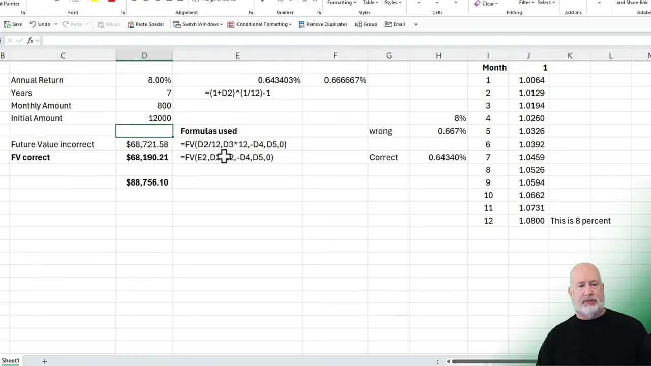

Validation checklist before you finalize

Use this quick checklist to validate your future value function results:

1. Confirm the monthly rate is (1+annual_rate)^(1/12)-1, not annual_rate/12.
2. Check that the sign of payments and present value follow Excel conventions (outflows negative).
3. Decide payment timing: beginning (1) or end (0) of period.
4. Compare Excel output to a reputable investment calculator for one or two simple scenarios (for example, $1 over 12 months should become 1+annual_rate).
5. If you use a named cell for the monthly rate, lock it with absolute references when copying formulas across cells.

Why this matters for long-term models

The difference between using annual_rate/12 and the compounded monthly rate may look small in a single month. Over multi-year horizons and recurring contributions, it compounds, producing differences that can mislead decisions about retirement planning, savings targets, or expected portfolio size.

Because I frequently build recurring contribution projections, I always compute the monthly equivalent rate explicitly and keep the formula transparent. It makes audits and explanations much easier and avoids subtle but material errors.

YouTube Video - Future Value

Summary

The future value function in Excel is powerful, but it requires the correct monthly rate when modeling monthly compounding. Use r_m = (1 + annual_rate)^(1/12) - 1, mind signs and timing, and validate with a calculator or a simple $1 test. Those few steps will make your projections reliable and defensible.

If you want a compact set of formulas to copy into your workbook, here are the essentials again:

MonthlyRate = (1 + AnnualRate)^(1/12) - 1
FV_Correct = FV(MonthlyRate, Years*12, -MonthlyContribution, -InitialBalance, PaymentTiming)
  

Apply those patterns, and your future value calculations will match real-world compounding every time.