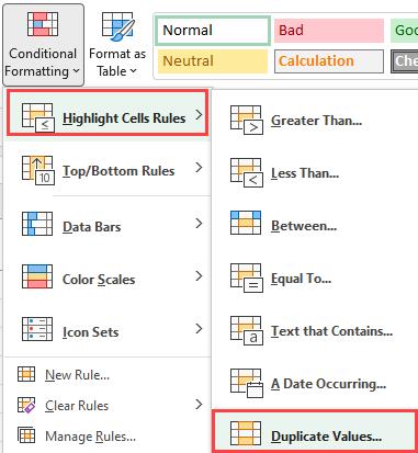
Excel - Find & Highlight Duplicate Rows - 3 Methods | Conditional Formatting

Posted on: 09/05/2021

Microsoft Excel can find duplicates easily with Conditional Formatting. The issue is Conditional Formatting finds duplicates based on the cell value, but I want to find duplicate rows. I use three methods in the video to find duplicate rows.

Excel conditional formatting - duplicates are based on cell value, not row values.

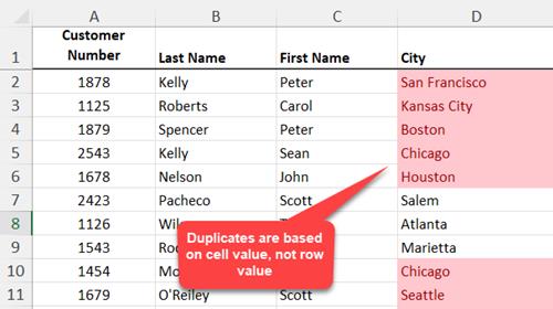
Duplicates using Conditional Formatting in Excel — Duplicates cell values using Conditional Formatting in Excel

In the video below, I start off with CONCATENATE, then use the TEXTJOIN function, and finally COUNTIFS with no helper column. To highlight the rows I use Conditional Formatting using a formula.

YouTube video

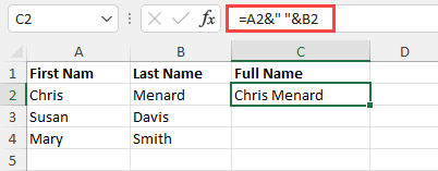
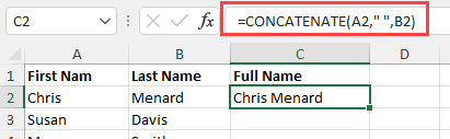
CONCATENATE in EXCEL

Method 1

Use CONCATENATE, one of the text functions, to join two or more text strings into one string. You can use an ampersand also which I use in the video.

Example: cell A2 has Chris and cell B2 contains Menard. =a2&" "&B2 will return Chris Menard in cells C2. Same example but using CONCATENTATE, you would type in cell C2, =CONCATENTATE(A2," ",B2) to get Chris Menard.

CONCATENATE Function in Excel — CONCATENATE Function

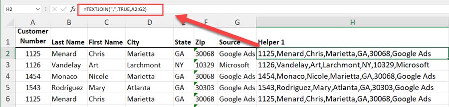
TEXTJOIN Function

Method 2

The TEXTJOIN function combines the text from multiple ranges and/or strings, and includes a delimiter you specify between each text value that will be combined. If the delimiter is an empty text string, this function will effectively concatenate the ranges.

Who has TEXTJOIN Function in Excel?

Office 2019 Windows
Office 2019 Mac
Microsoft 365 subscriber

Conditional Formatting with COUNTIFS Function

Method 3

The two methods I used earier - CONCATENTATE and TEXTJOIN - required a helper column. This 3rd method uses Conditional Formatting with the COUNTIFS function. This is the longest method, but a helper column in not required.

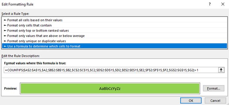
The formula I wrote for COUNTIFS inside on Conditional Formatting is
=COUNTIFS($A$2:$A$15,$A2,$B$2:$B$15,$B2,$C$2:$C$15,$C2,$D$2:$D$15,$D2,$E$2:$E$15,$E2,$F$2:$F$15,$F2,$G$2:$G$15,$G2)>1

Steps

Select A2 to G15 or the range.
Click Conditonal Formatting - New Rule.
Select Use a formula to determine which cells to format.
Type the function above or copy and paste it.
Click Format and pick a color.
Click OK twice.

Conditional Formatting with COUNTIFS for Duplicate Rows

Chris Menard

Chris Menard is a certified Microsoft Trainer (MCT) and works as a full-time Trainer at BakerHostetler - one of the largest law firms in the US. He runs a YouTube channel with 900+ technology videos that cover various tools such as Excel, Word, Zoom, Teams, Gmail, Google Calendar, and Outlook. To date, the channel has helped over 20 million viewers. Menard also does 2 to 3 public speaking events every year, presenting at the Administrative Professional Conference (APC), the EA Ignite Conference, the Support Staff Conference, the University of Georgia, and CPA conferences. You can connect with him on LinkedIn at https://chrismenardtraining.com/linkedin or watch his videos on YouTube at https://chrismenardtraining.com/youtube.