Excel AVERAGE excluding the highest and lowest values | TRIMMEAN Function

When you have a range of numbers in Excel and want to figure out the AVERAGE but you have some extreme values that can skew your averages, there is a function that helps solve that problem.

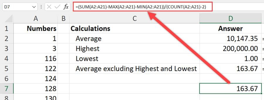
**Average using Sum with Max, Min, and Count**

You can calculate the AVERAGE in Excel using the TRIMMEAN function, which will allow you to exclude lowest or highest values from being considered for the averages. Further, you can exclude one or more highest/lowest values in your range, by specifying how many you want to ignore.

In this article and video I walk you through several methods of calculating this average, using the classic AVERAGE function, then using the MIN and MAX functions to exclude values from consideration, and finally, I show you the TRIMMEAN function in a formula, to exclude extreme values automatically from your averages.

YouTube video

Excel AVERAGE excluding the highest and lowest values | TRIMMEAN Function

Method 1 - Average with Max and Min Functions

To find the average and exclude the highest and lowest number, we can sum the range of number, subtract the max and min, which are the highest and lowest, and divide by the couunt of the numbers minus 2. See the screenshot at the top of this post.

Method 2 - Use the TRIMMEAN Function

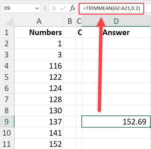
**TrimMean Function in Excel**

The TRIMMEAN function has two arguments. Both are required argument. In my example, I have 20 numbers that go from A2 to A21. The percentage is 10% or .1 in my example Twenty numbers times 10% is 2. Two numbers are excluded from the mean. The two numbers are the largest and the smallest.

If I made the percentage 20%, that would be four numbers, 20 x  2%=4. The Average would exclude the top two highest and the lowest two numbers from the average.

Syntax

TRIMMEAN(array, percent)