How to Combine UNIQUE, CHOOSECOLS, COUNTA, and SORT in Excel

If you analyze data in Excel, the UNIQUE function is one of the quickest ways to cut through noise and see exactly what you have. I rely on UNIQUE every day, and when I pair it with SORT, COUNTA, and CHOOSECOLS, it becomes a powerful tool for cleanup and analysis. Below, I’ll show practical examples and share a few bonus tips that remove manual work and help you catch messy data before you run calculations or PivotTables.

Quick overview: When to use UNIQUE

Use UNIQUE whenever you need a list of distinct values from a column or a set of columns. It works on single columns, adjacent columns, and—when combined with CHOOSECOLS—non-adjacent columns too. UNIQUE is available to Microsoft 365 users on Windows, Mac, and Excel for the web.

Training File for Unique SORT CHOOSECOLS

Basic examples and common combinations

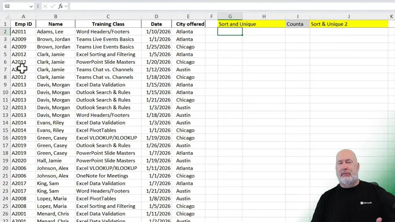
Extract a single column of unique values

The simplest form returns a spill array with all distinct entries from a range:

=UNIQUE(A2:A53)

If the list updates frequently, UNIQUE keeps the output dynamic. No more manual copying or counting.

Sort the unique results

Wrap UNIQUE inside SORT to automatically get an ordered list. This is handy for alphabetical reports or for cleaning up messy lists before analysis.

=SORT(UNIQUE(A2:A53))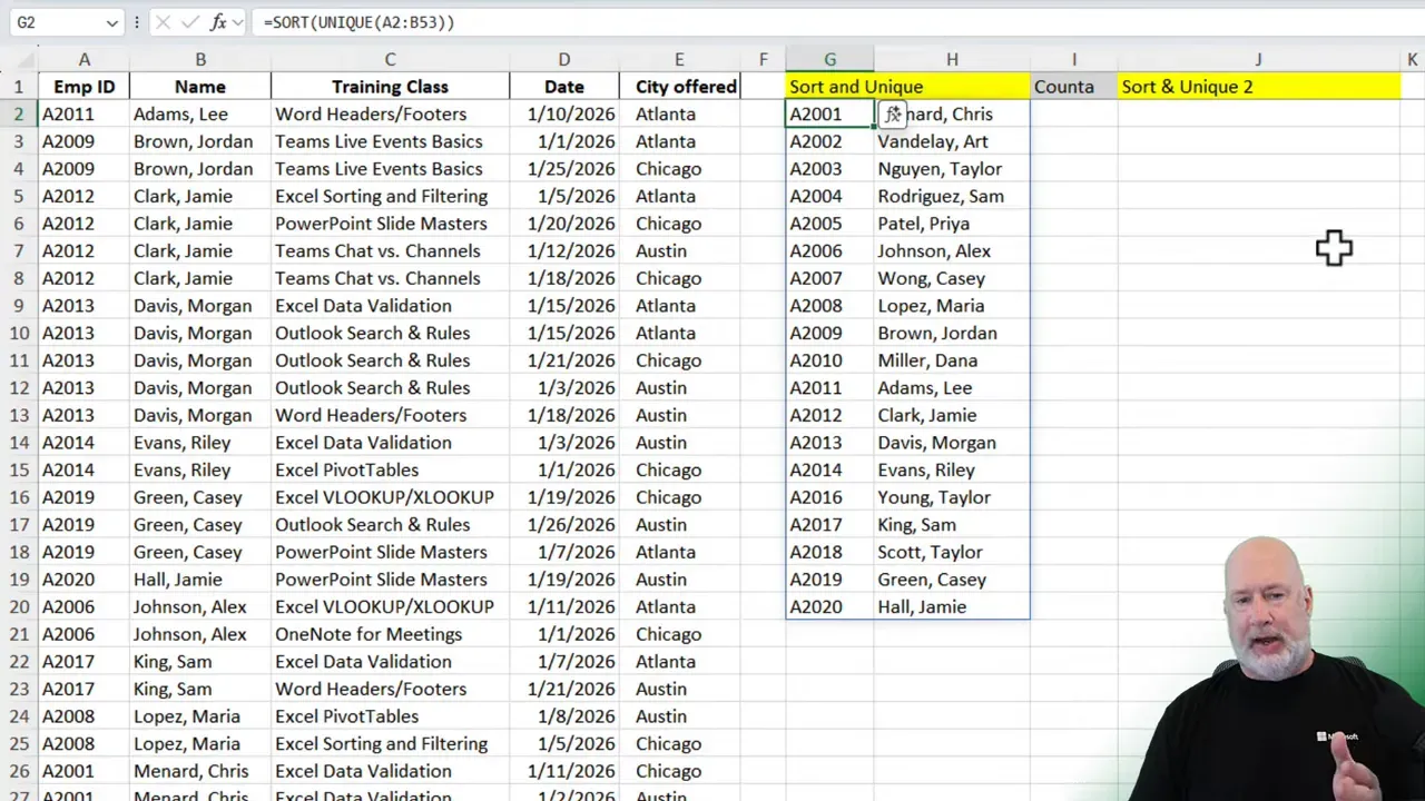

Count the number of unique items

If you want a dynamic count of distinct entries, nest UNIQUE inside COUNTA. COUNTA counts both text and numbers and reflects changes in the source data.

=COUNTA(UNIQUE(A2:A53))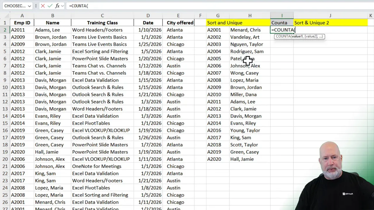

Problem: pulling non-adjacent columns

UNIQUE works perfectly with adjacent columns (for example, A2:B53). But what if the columns you need are not next to each other? You might want the employee ID from column A and the city from column E. Selecting A2:A53 and E2:E53 directly inside UNIQUE will return an error.

Solution: CHOOSECOLS

CHOOSECOLS lets you pick specific columns from a multi-column range and return a new array containing only those columns. Use it to create a virtual, compact table you can feed into UNIQUE.

=CHOOSECOLS(A2:E53, 1, 5)

That returns two columns: column 1 and column 5 from the original range. Now wrap that inside UNIQUE.

=UNIQUE(CHOOSECOLS(A2:E53, 1, 5))

If you want those results sorted as well, nest with SORT:

=SORT(UNIQUE(CHOOSECOLS(A2:E53, 1, 5)))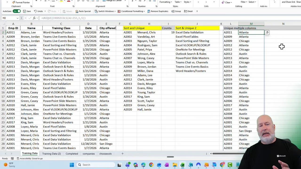

Use cases: cleaning and preparing data before analysis

Before creating PivotTables or calculating revenue by company, I always check for inconsistent labels. UNIQUE plus SORT is a fast way to spot duplicates that are not truly duplicates—things like extra spaces, alternate names, or inconsistent capitalization.

For example, "JPMorgan Chase" and "JPMorgan Chase" (two spaces) look similar but will be treated as different entries. A quick, sorted, unique list highlights those issues so you can fix them first.

Practical cleanup flow

1. Run SORT(UNIQUE(range)) on the company or ID column.
2. Scan the list for inconsistent names or spacing.
3. Standardize names with TRIM, UPPER/LOWER, or a lookup table if needed.
4. Proceed to PivotTables or calculations on cleaned data.

Bonus tip: Highlighting uniques with Conditional Formatting

Conditional Formatting can show duplicates or unique values. If you expect duplicates and want to quickly spot the unique entries, choose Highlight Cells Rules → Duplicate Values and select the Unique option. That highlights the single-occurrence entries so you can filter and inspect them.

After highlighting, right-click a highlighted cell and choose Filter → Filter by Selected Cell Color to isolate those rows. This technique is great for visual QA before you run summaries.

Examples and quick reference

• Unique list from one column — =UNIQUE(A2:A100)
• Sorted unique list — =SORT(UNIQUE(A2:A100))
• Count distinct values — =COUNTA(UNIQUE(A2:A100))
• Unique rows from non-adjacent columns — =UNIQUE(CHOOSECOLS(A2:E100,1,5))
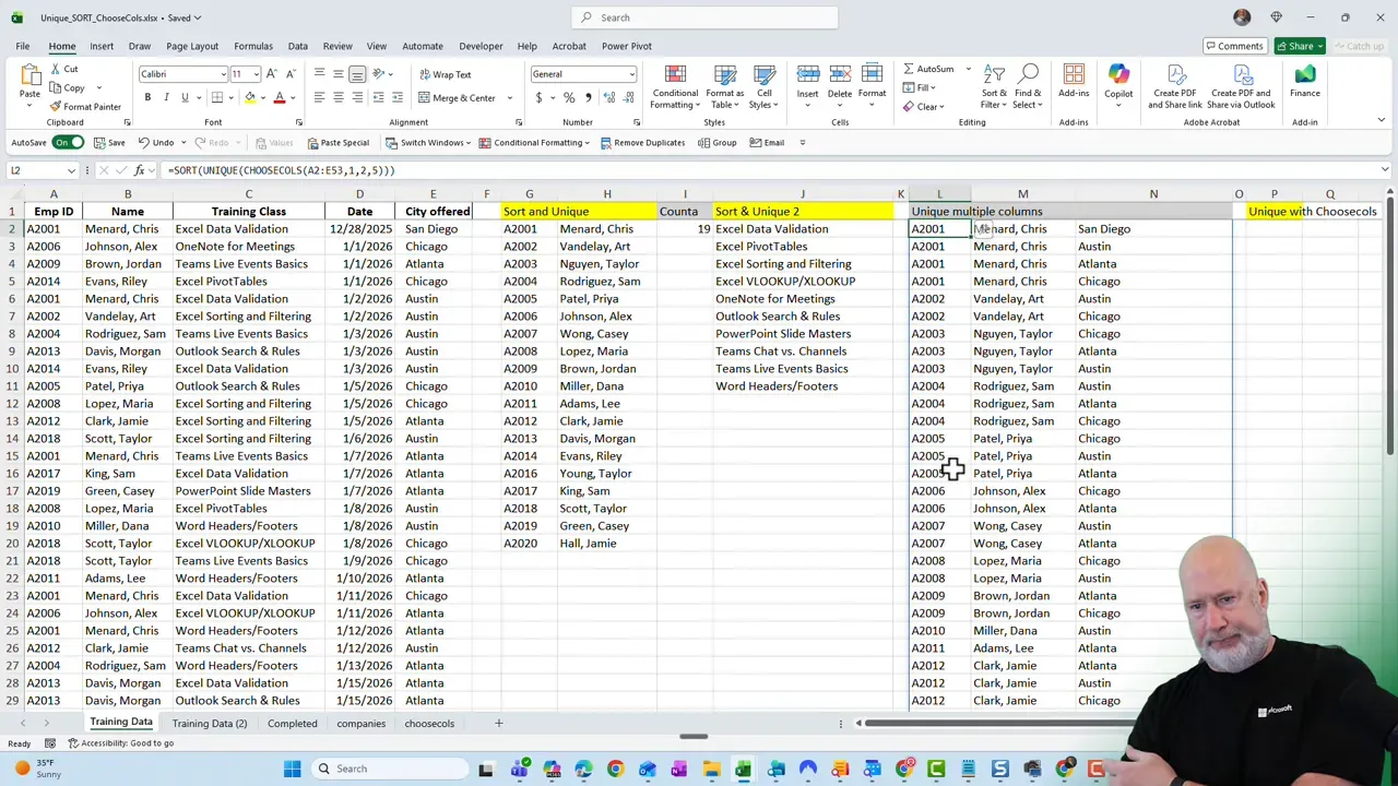
• Sorted unique from non-adjacent — =SORT(UNIQUE(CHOOSECOLS(A2:E100,1,2,5)))

When UNIQUE does not behave as expected

A few common pitfalls:

• Hidden trailing spaces. Use TRIM to normalize text.
• Different casing. Use UPPER or LOWER to standardize.
• Mixed data types in one column. Convert numbers stored as text or vice versa.
• Using UNIQUE on nonspillable ranges. Ensure there is space below the cell for the spill array to appear.

YouTube Video

What Excel versions include UNIQUE, SORT, COUNTA, and CHOOSECOLS?

UNIQUE, SORT, and CHOOSECOLS are part of the dynamic array functions available to Microsoft 365 subscribers. COUNTA is an older function available in all modern Excel versions.

Can UNIQUE handle multiple columns?

Yes. UNIQUE can accept multiple adjacent columns as a single range (for example A2:B53). For non-adjacent columns, use CHOOSECOLS first to assemble the columns you want.

How do I count unique rows where more than one column matters?

Combine UNIQUE on a multi-column range with COUNTA or use COUNT(UNIQUE(...)) depending on whether you need a numeric or textual count. For non-adjacent columns, use CHOOSECOLS inside UNIQUE.

What’s the best way to find inconsistent entries before analysis?

Generate SORT(UNIQUE(range)) to get a compact, ordered list of values. Scan for variations such as extra spaces, abbreviations, or alternative naming. Use the TRIM and TEXT functions, or a mapping table, to standardize names before summarizing.

Final notes

UNIQUE, when combined with SORT, COUNTA, and CHOOSECOLS, reduces the number of manual steps in data cleanup and analysis. Use these functions to:

• Generate dynamic lists of distinct values
• Count distinct items without manual selection
• Pull non-adjacent columns into tidy arrays
• Spot and fix inconsistent data before running reports

Once you start using these combinations, you’ll find fewer surprises in your PivotTables and summaries and spend less time cleaning data and more time analyzing it.