Find the lowest / highest values for rows or columns with conditional formatting in Excel

You can find the lowest or highest values for rows or columns in Excel using Conditional Formatting. You will need to use eihter the MIN Function, which finds the lowest value, or the MAX function, which finds the highest value.
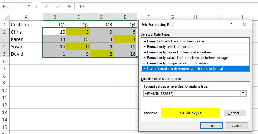
To find the lowest value by Rows
1. Select your range 2. Make sure you are on the **Home** Tab. 3. Click **Conditoinal Formatting,** then **New Rule.** 4. Click **Use a formula to determine which cells to format.** 5. Type **=B2=MIN($B2:$E2)** then click **Format** \- **Fill** tab - pick a color. 6. Click **OK**.
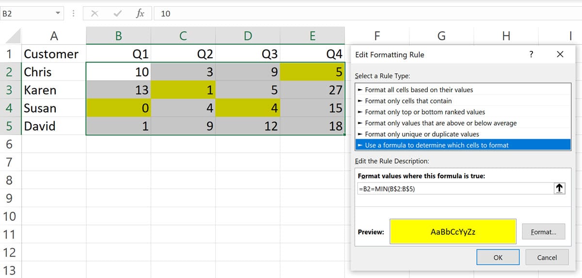
To find the lowest value by Columns
1. Select your range 2. Make sure you are on the **Home** Tab. 3. Click **Conditoinal Formatting,** then **New Rule.** 4. Click **Use a formula to determine which cells to format.** 5. Type **=B2=MIN(B$2:B$5)** then click **Format** - **Fill** tab - pick a color. 6. Click **OK**.
Excel: find the lowest/ highest values for rows or columns w/ conditional formatting by Chris Menard
Other videos on Conditional Formatting
[Conditional Formatting with Dates](http://anything%20over%2030%20days%20you%20want%20in%20a%20yellow%20background%20and%20anything%20over%2060%20in%20a%20green%20background.%20you%20will%20use%20the%20today%20function%20in%20excel%20with%20conditional%20formatting./)
Anything over 30 days you want in a yellow background and anything over 60 in a green background. You will use the TODAY function in Excel with Conditional Formatting.
[Conditional Formatting with the AND Function](
To use Conditional Formatting based on two conditions in Excel, use the AND function.
=AND($E2="CA",$F2="Google Ads") to find people in CA that found you through Google Ads.