Combine Excel's UNIQUE, LEFT, SEARCH & SORT Functions

What I'm trying to solve 🧩

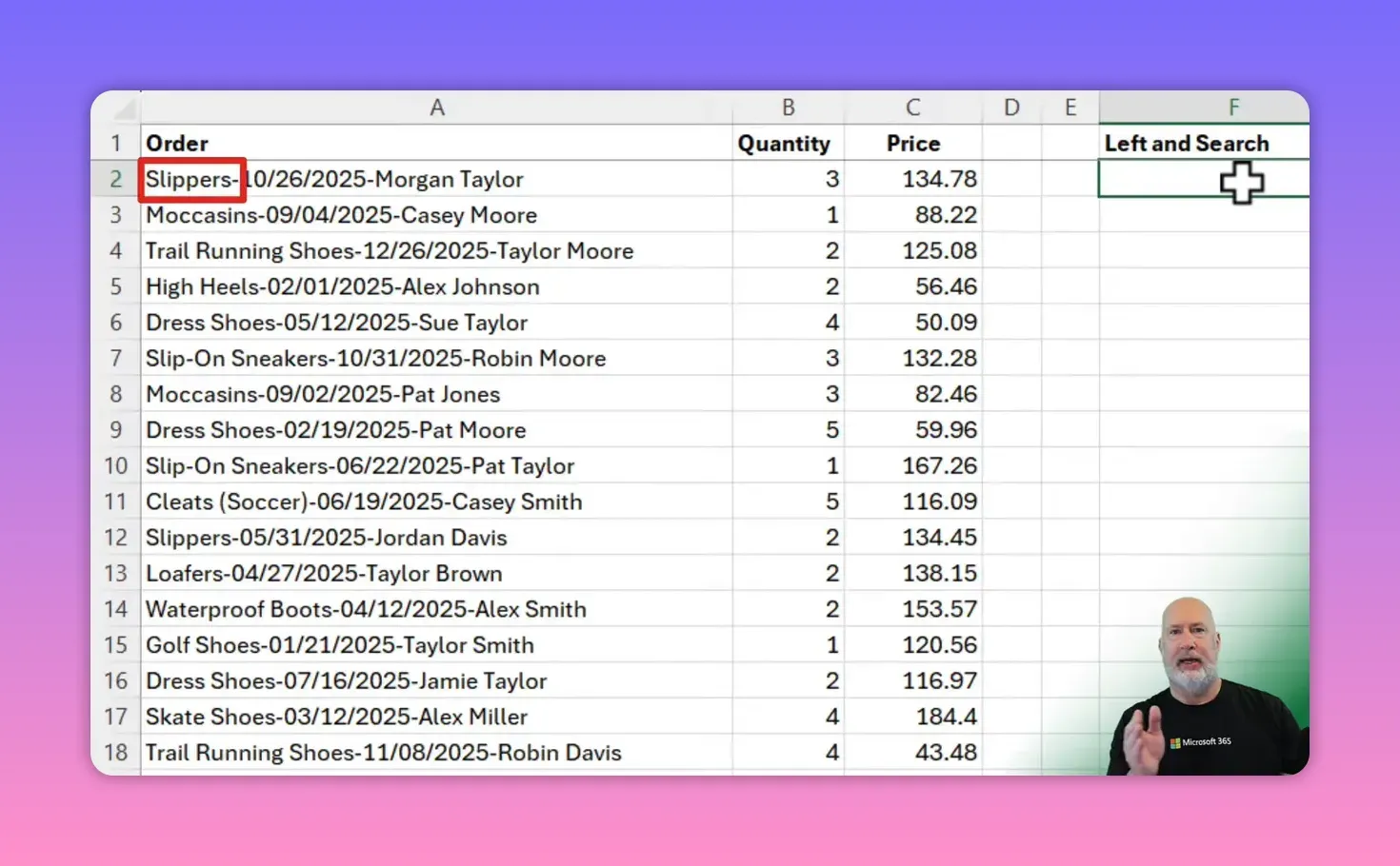
I had a column of 100 order lines, with each line beginning with the product name, then the order date, then the customer name. My goal was simple: show each product only once. Duplicate products appear throughout those 100 rows, and the product name sits at the start of the text in each cell. A few quirks in the text led me to combine functions rather than rely on a single extraction function.

Why TEXTBEFORE looked promising but failed ⚠️

TEXTBEFORE is elegant when the delimiter is consistent. My first thought was to use it to grab everything before the date. The basic syntax is short and easy to read, and when it works it works fast. TEXTBEFORE and TEXTAFTER are two of my favorite Excel functions, but they don't work for this example.

TEXTBEFORE syntax
TEXTBEFORE(text, delimiter, [instance_num], [match_mode], [match_end])

For many cells it returned the expected product. But some product names contain characters or spacing that make a simple delimiter selection unreliable. For example, when a product name contains a hyphen or an unexpected spacing pattern, picking a single delimiter like a space or comma returned only the first word ("slip" from "slip-on sneakers"). That taught me to always check the data before settling on a delimiter-based extraction method.

Excel TEXTBEFORE and TEXTAFTER to Extract Data from Strings

YouTube video

LEFT function explained ⬅️

The LEFT function returns a specified number of characters from the beginning of a text string. It's predictable and works perfectly when you know how many characters you need. The trick is calculating that character count dynamically.

LEFT syntax
LEFT(text, num_chars)

Example: LEFT("slippers / 10/26/2025", 8) returns "slippers". The challenge is that product name lengths vary, so hard-coding the num_chars is not viable across the full range.

YouTube Video - Combine Excel's UNIQUE, LEFT, SEARCH & SORT Functions

SEARCH function explained 🔎

SEARCH finds the position of a character or substring inside a text string. Use SEARCH to locate the boundary between the product name and the date, then feed that position into LEFT to pull the product name.

SEARCH syntax
SEARCH(find_text, within_text, [start_num])

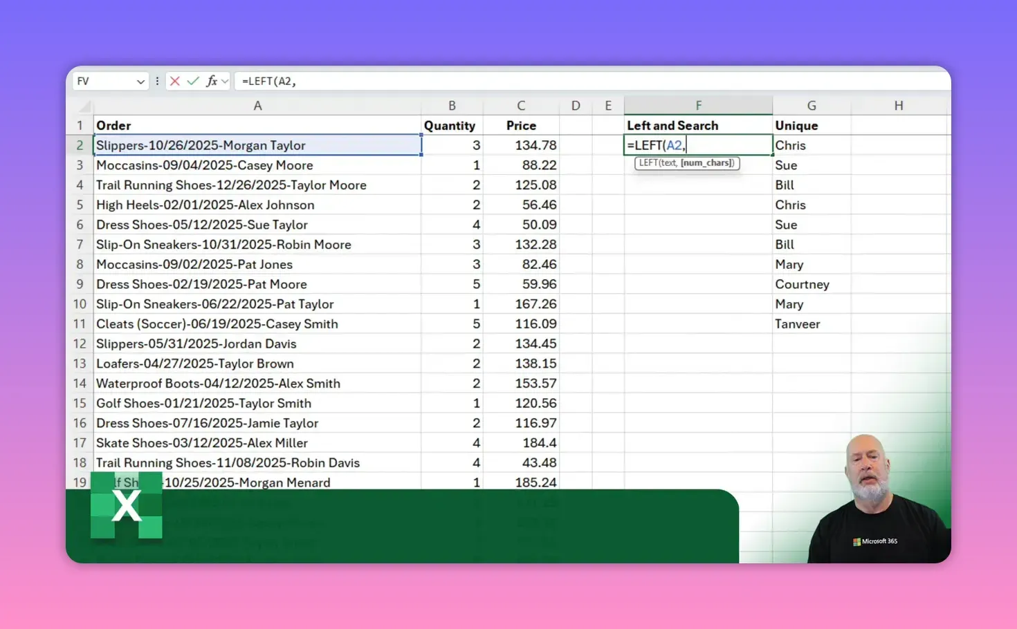
If the date always starts after a specific separator (for example a forward slash or a consistent pattern), SEARCH will return the character index of that separator. In my data the date format used two-digit months consistently, and a reliable marker existed a few characters after the product name.

When using SEARCH inside LEFT you subtract a small number to remove the separator and any trailing spaces or symbols. In my case I subtracted four characters to remove the slash and spacing, so this pattern worked:

Example formula (cell A2)
LEFT(A2, SEARCH("/", A2) - 4)

Note: the number you subtract depends on the exact characters that appear between the product name and the date. Always inspect a few sample rows before committing to a subtraction value.

UNIQUE function explained 🔢

UNIQUE is the function that filters a list down to distinct values. Use it after you’ve extracted product names so duplicates collapse into a single list.

UNIQUE syntax
UNIQUE(array, [by_col], [exactly_once])

Common usages:

• UNIQUE(A2:A101) returns every distinct value from the range.
• UNIQUE(A2:A101,,TRUE) returns only the items that appear exactly once in the range.
• Remember you can use UNIQUE on the results of another formula, such as LEFT combined with SEARCH.

Putting LEFT, SEARCH and UNIQUE together 🧰

Once I had a working LEFT+SEARCH extraction for each row, the next step was to apply UNIQUE to the whole extracted range. Because modern Excel supports dynamic arrays, I could write a single nested formula that returned a spill range of distinct product names.

Combined extraction and uniqueness
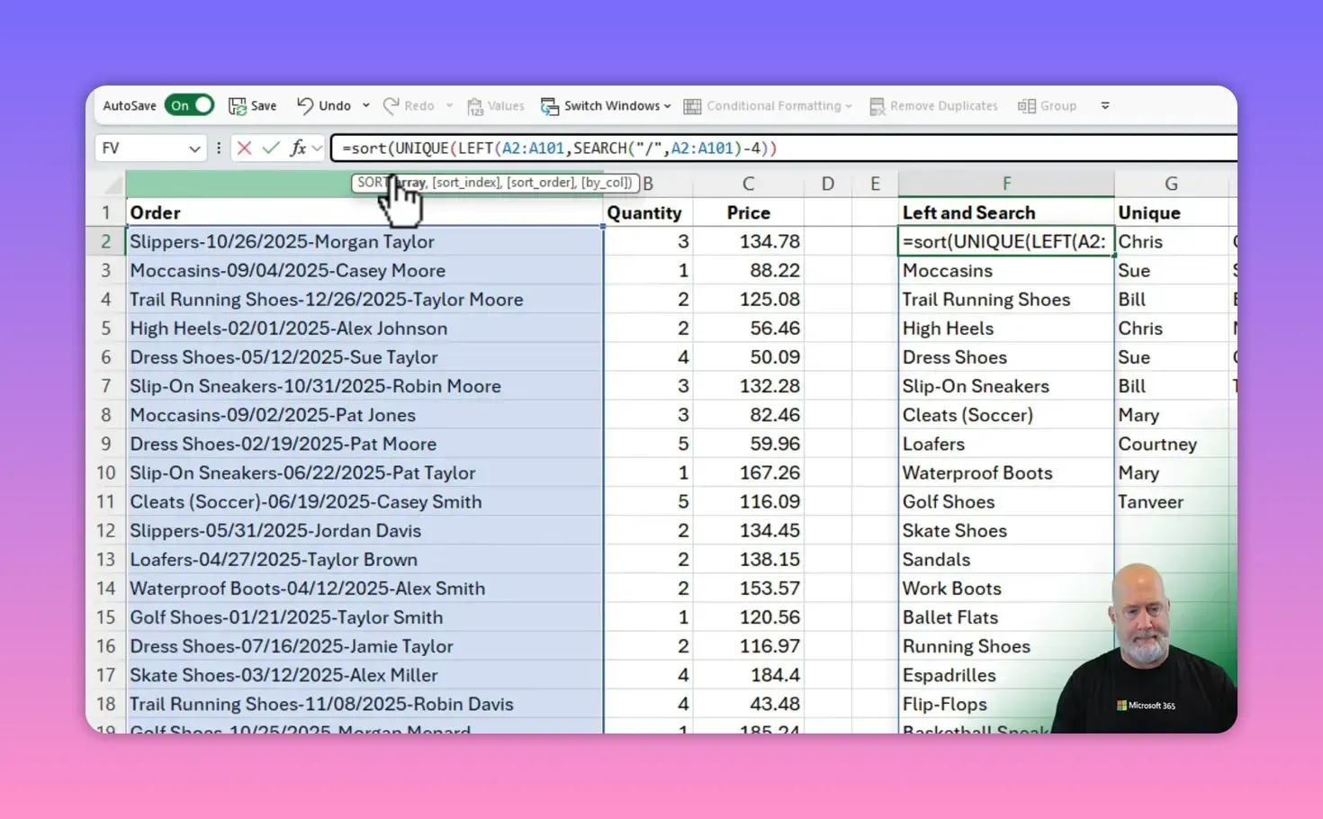
UNIQUE(LEFT(A2:A101, SEARCH("/", A2:A101) - 4))

This formula does three things in one shot:

1. SEARCH finds the separator position for every cell in A2:A101.
2. LEFT extracts each product name based on those positions.
3. UNIQUE removes duplicate product names and spills the distinct list into adjacent cells.

Make sure the SEARCH pattern (for example "/") actually exists consistently. If not, tweak the SEARCH target or consider preprocessing the raw text.

Sorting the final list 🔀

A neat final touch is wrapping SORT around the UNIQUE call so the unique list appears alphabetically or in another predictable order. That’s how I shared a clean, alphabetized list with my team lead.

SORT + UNIQUE example
SORT(UNIQUE(LEFT(A2:A101, SEARCH("/", A2:A101) - 4)))

After the formula spills and I confirm the results, I typically copy the spill range and paste values to produce a static list to hand off to others.

Practical tips and troubleshooting 🛠️

• If TEXTBEFORE returns only the first word, try a different delimiter or fallback to LEFT+SEARCH.
• Always inspect several rows for variations like hyphens, extra spaces, or alternate punctuation.
• If the separator is inconsistent, consider using helper columns to clean or standardize the separator first, or use more advanced text functions or Power Query.
• Use UNIQUE with the exactly_once argument to find rare, single-appearance products: UNIQUE(range,,TRUE).

How do I choose between TEXTBEFORE and LEFT plus SEARCH?

If there is a single, consistent delimiter that never occurs in the product name, TEXTBEFORE is clean and simple. If the delimiter is inconsistent or the product name itself can contain the delimiter (for example spaces or hyphens), LEFT combined with SEARCH gives you better control because you can fine-tune the character offset.

What exact formula did I use to extract product names?

I used LEFT together with SEARCH to find the product boundary and then UNIQUE to collapse duplicates. For my dataset the working formula was: UNIQUE(LEFT(A2:A101, SEARCH("/", A2:A101) - 4)). Finally I wrapped SORT around that for an alphabetized result.

What if the separator is a comma or another character?

Replace "/" in the SEARCH call with the actual separator character. For example SEARCH(",", A2) or SEARCH(" - ", A2). Adjust the subtraction value to remove trailing punctuation or spaces. Always test on several rows first.

How do I count the unique items once I extract them?

Wrap COUNT or COUNTA around the UNIQUE spill. Example: COUNTA(UNIQUE(LEFT(A2:A101, SEARCH("/", A2:A101) - 4))). That returns the number of distinct products.

Closing thoughts ✨

When text is predictable, simple functions like TEXTBEFORE shine. When the data contains inconsistent spacing, hyphens, or additional punctuation, combining SEARCH and LEFT gives the fine-grained control needed to extract the right substring reliably. Pair those extraction methods with UNIQUE, and then SORT for presentation, and you have a robust workflow for turning messy order lines into a clean list of products.