Microsoft Excel

Use Icon Set in Excel - just two arrows by Chris Menard

Chris Menard

10 Feb 2017 — 1 min read

Icon Sets in Excel

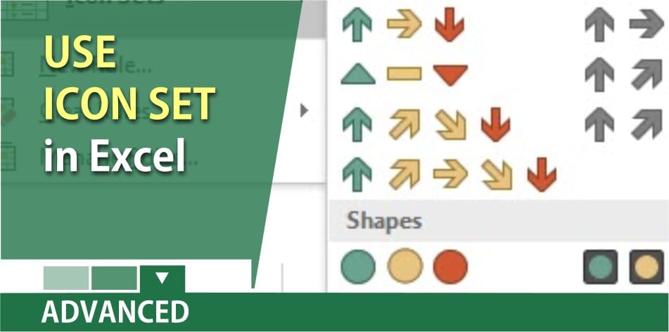
Use an icon set to present data in three to five categories that are distinguished by a threshold value. Each icon represents a range of values and each cell is annotated with the icon that represents that range. For example, a three-icon set uses one icon to highlight all values that are greater than or equal to 67 percent, another icon for values that are less than 67 percent and greater than or equal to 33 percent, and another icon for values that are less than 33 percent.

In the video below, I only want to use the green arrow point up for positive numbers, and the red arrow pointing down for negative numbers. I do not want to use the yellow arrow. When showing icon set arrows, the arrows appear to the left of the number. You can not display the number and the arrows will appear in the middle of the column as shown in the video below.

Use two arrow icon set with conditional formatting in Excel by Chris Menard -

Chris Menard to Present “Executive Insights: Harnessing Excel for Strategic Analysis” at EA Ignite Conference

November 4, 2025 Microsoft MVP and productivity expert Chris Menard will be presenting a highly anticipated session titled “Executive Insights: Harnessing Excel for Strategic Analysis” at the EA Ignite Conference, held at the Renaissance Nashville Hotel. This premier event, running from November 3–5, 2025, is tailored for executive assistants

Chris Menard to Present “Mastering Microsoft 365 Copilot” at EA Ignite Conference

Chris Menard will present “Mastering Microsoft 365 Copilot” at EA Ignite in Nashville on Nov 3, 2025. Learn how Copilot boosts productivity in Word, Excel, PowerPoint, Outlook, and Teams during this hands-on session.

Microsoft Teams: Save Chat and Channel Messages is Back!

How to use the newly returned feature that lets you save Chat and Channel Messages in Teams so you can keep important conversations at your fingertips.

OneDrive Request Files: How to Use OneDrive to Collect Files Securely

OneDrive Request Files feature allows you to collect files from people inside or outside your organization, without letting those people see anyone else’s uploads.