Microsoft Excel

Conditional Formatting with two criteria using AND function in Excel

Chris Menard

02 Apr 2017 — 1 min read

Conditional formatting is one of my favorite features in Excel. I like it because I’m a visual person. Excel has a lot of predefined rules in Conditional Formatting, but it is very easy to write a formula if the predefined rules don’t have what you need. An Executive MBA student from the University of Georga wanted to know how to highlight the entire row in Excel based on two conditions instead of one condition. Now is the time to use the **AND** function in Excel.

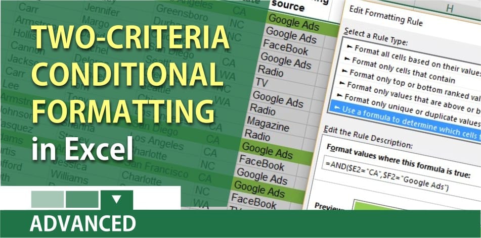
The exercise I used was to find people in California, abbreviated as CA in our data, that found use through Google Ads.

Steps to use the AND Function in Conditional Formatting:

Select the row below the header row to the end of your data. In the screenshot, I started selecting from A2.

1. On the Home tab, click **Conditional Formatting** in the Styles group.

2. Click New Rule.

3. Click **Use a formula to determine which cells to format**.

4. Click in the formula area and type **=AND($E2=”CA”,$F2=”Google Ads”)**

5. Click **Format** and click the **Fill** tab.

6. Pick Yellow or Orange and click **OK** twice.

Excel file used in this example and video [Subtotals – Chris Menard](https://chrismenardtraining.com/wp-content/uploads/2017/04/Subtotals-Chris-Menard.xlsx)

YouTube video of Conditional Formatting with two criteria

Conditional Formatting with the AND function in Excel

More information about Conditional Formatting

- Chris Menard shows how to use [conditional formatting with groups of data](

- [Conditional Formatting with dates in Excel](

- [Conditional Formatting](

with Countif in Excel

OneDrive Recycle Bin Tips and Tricks: How to Recover Files

I rely on OneDrive every day, and the OneDrive Recycle Bin is one of those quiet lifesavers most people forget about until they panic. Whether it's a Teams meeting recording that a policy removed after 60 days or a spreadsheet I accidentally deleted, knowing how the OneDrive Recycle

Combine Excel's UNIQUE, LEFT, SEARCH & SORT Functions

What I'm trying to solve 🧩 I had a column of 100 order lines, with each line beginning with the product name, then the order date, then the customer name. My goal was simple: show each product only once. Duplicate products appear throughout those 100 rows, and the product

Count Unique Values in Excel with UNIQUE, SORT, and COUNTIF Functions Tutorial

Table of Contents * 📋 Why this method works and when I use it * 📋 Setting up the table * 🔎 Extract distinct values with UNIQUE * ↕️ Sort the unique list with SORT * 🔢 Count occurrences using COUNTIF * ✅ Why tables beat ranges for this task * 🔁 When to use this instead of a pivot table * 🔧 Quick checklist to

Financial Ratios - Formula Completion in Excel using Copilot

Writing formulas in Excel can be time-consuming and challenging, even for experienced users. Selecting the right function, referencing the correct cells, and ensuring proper syntax often slows down workflows and leads to errors. Many users spend extra time troubleshooting mistakes, searching for examples, or trying to recall the exact formula