Compare two lists or columns in Microsoft Excel

If you need to compare two lists or columns in Microsoft Excel, you can either use Conditional Formatting or you can you an empty column and use Countif function. You can even use both. This is handy when you want to compare 2016 customers to 2017 customers or a list of employees or products.

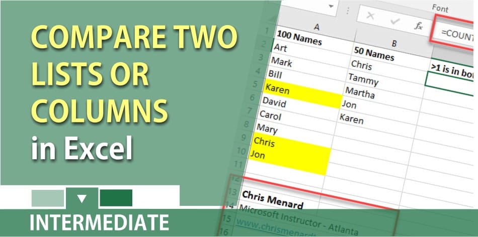
To compare the master list, let’s assume this is column A and you have a new list which is column B and you want to see who is already in Column A that is in Column B, let’s use Conditional Formatting first.

1. Select A2 to A10. 2. Click Conditional Formatting, Click New Rule. 3. Click Use a formula to determine which cells to format. 4. Type in the formula =Countif($A$2:$A$10,$B2). 5. Click Format. 6. Click Pattern and pick yellow. 7. Click OK. 8. Type another name in column B to test it.

Two screenshots below

This is the end result. Notice Tammy and Martha are not in the master list

This is the function you will type in the Conditional Formatting box

YouTube video on comparing two columns or lists

Find duplicates and compare two lists in Microsoft Excel by Chris Menard