Advanced Excel Conditional Formatting with Mixed and Absolute References

The Power of Conditional Formatting
In this blog post, we will explore the concept of Conditional Formatting in Microsoft Excel. Conditional formatting is a powerful feature that allows users to highlight cells that meet specific criteria, highlight numbers over or below the average, and use Data Bars. By using conditional formatting, you can quickly identify and analyze data that meets particular requirements.
Conditional Formatting Categories
- Highlight Cells Rules - Greater Than, Less Than, Between, Equal To, Text that Contains, A Date Occurring, Duplicate Values - Top/Bottom Rules - Top 10 Items, Top 10%, Bottom 10 Items, Bottom 10%, Above Average, Below Average - Data Bars - Different gradient fills. - Color Scales - Different colors. - Icon Sets - Use arrows and traffic signs, such as red, yellow, and green colors. - New Rule - write a formula. - Clear Rules - Clear rules from the worksheet or a range - Manage Rules - Edit Rules
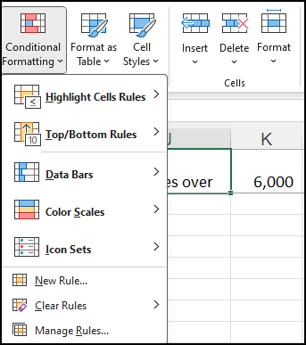
**Conditional Formatting in Excel**
Finding Numbers Over 6,000 - Highlight Cells Rules
Let's dive into an example to understand how conditional formatting works. Imagine you have a spreadsheet labeled "Purchases" (column H), and you want to find all the numbers over 6,000. Usually, users would use the "Highlight Cells Rules" feature under the "Conditional Formatting" tab to accomplish this.
Most users do this with conditional formatting by selecting cell H2 and pressing CTRL + SHIFT + down arrow to select all the numbers in column H. Then, navigate to the "Conditional Formatting" option under the "Home" tab. Select "Highlight Cells Rules" and "Greater Than" from the dropdown menu. Enter the number 6,000 as the threshold. Click "OK," and all the numbers over 6,000 will be highlighted.
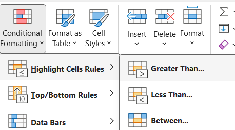
Highlight Cells Rules

Conditional Formatting over 6,000
YouTube Video
Advanced Excel Conditional Formatting with Mixed and Absolute References - YouTube
Conditional Formatting-Mixed & Absolute Reference
The Benefits of Mixed and Absolute References
Now, let's explore the alternative method using mixed and absolute references. Start by removing the previous conditional formatting by selecting "Clear Rules" and "Clear Rules from Entire Sheet." Next, insert the number 6,000 somewhere on your spreadsheet; in this example, it is placed in cell K1.
To apply conditional formatting using mixed and absolute references, select cell H2 again and press CTRL + SHIFT + down arrow to select all the numbers in column H. Instead of using the "Highlight Cells Rules" feature, we will create a new rule using a formula. Choose the option "Use a Formula to Determine Which Cells to Format." In the formula bar, enter **"=$H2=$K$1"** (without the quotes). We will only look at column H, starting in H2, and working down column H, which is the mixed reference, the $ in front of the letter H, and we will only reference cell K1, which is an absolute reference since it has two dollar signs.
After entering the formula, click on the "Format" button. You can choose any formatting options, such as changing the cell's fill color to green. Once you have made your formatting selections, click "OK" twice.
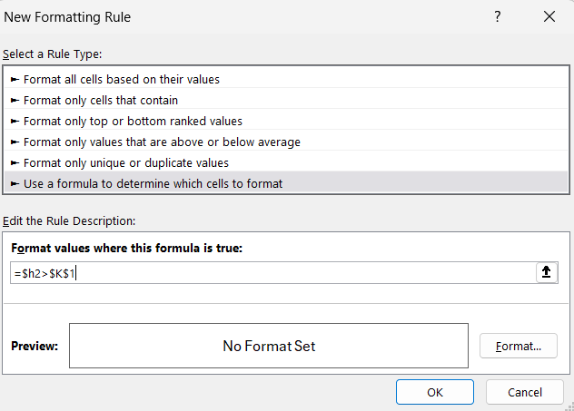
Conditional Formatting with Mixed and Absolute Reference
The Advantages of Using Mixed and Absolute References
So, what makes the method using mixed and absolute references better? Firstly, it provides clarity and transparency. By explicitly stating that you are looking for "Purchases Over 6,000" in cell K1, anyone who views the spreadsheet can easily understand the conditional formatting's purpose.
Additionally, using mixed and absolute references allows for quick and easy adjustments. If you decide to change the threshold from 6,000 to 5,500, you only need to modify the value in cell K1. The conditional formatting will automatically update to reflect the new criteria, saving you time and effort.
