DeKalb Chapter of The Georgia Society of CPAs
Excel Analysis and PivotTables


Date: Tuesday, February 25, 2020

The chapter meeting is from 5:00 pm to 7:30 pm at Petite Violette

5:30 pm to 6:20 pm is Chris Menard's presentation

Chris Menard

Hi, I'm Chris Menard and I'll be your instructor for Excel Analysis and PivotTables

I'm a member of the Microsoft Creator team and my public speaking client list includes The Georgia Society of CPAs for over 10 years, the Continuing Education Center for the University of Georgia since 2009, the Executive MBA students at the University of Georgia since 2010, and many others. In my spare time, when I’m not keeping up to date with the latest MS Office 365 features, I provide free support and create video tutorials on software topics and issues. My YouTube channel is approaching 500 training videos and many of my training videos are on Microsoft's YouTube Channel.

Topics I will be covering: 
PivotTables, Charts, Web Data,
Text vs Number, Tables.

See below some videos with sample topics.
GSCPA logoLocation: 
Petite Violette
DeKalb County: Map
Signup for this event


Here are some videos related to the topics we'll be discussing:


Show Report Filter Pages with PivotTable

Excel PivotTables
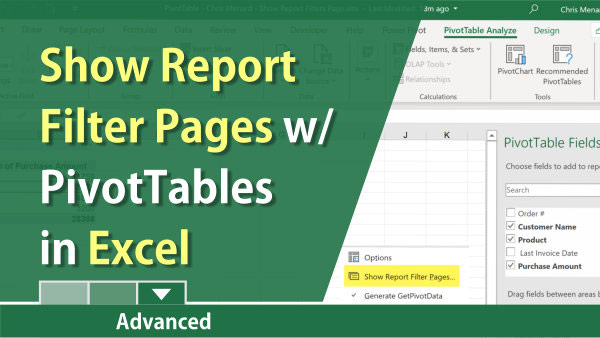
Show Report Filter Pages: Create Many PivotTables at Once

Excel has a great feature that allows you to create multiple PivotTables from one PivotTable. It is called "Show Report Filter Pages."  

To use this feature, you have to use the Filter area in a PivotTable. The field you want to drag to the Filter area of the PivotTable is the field you wish to create many PivotTables. 

As an example, if you want each Sales Rep to have their own PivotTable report, and you have a field called Sales Rep, you would drag Sales Rep to the filter area. You need two other fields. Most likely, one is in the row area, and the other field, usually numeric, is in the values areas.

Watch this video

Edit the default layout of PivotTables in Excel

Excel PivotTables
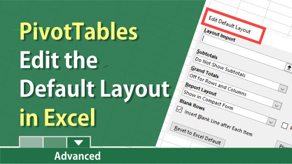
Change the default layout of a PivotTable

You can change the default layout for PivotTables. You can add blank rows, show subtotals at the bottom, and only show grand totals for rows or columns. This is only available with an Office 365 subscription or Office 2019. It is not available with Office 2016.  

If you go to File - Options and see the Data category, this feature is available. If not, this feature is not available. Here is a screenshot of the data category.

Watch this video

Create a PivotTable from multiple worksheets in Excel

Excel PivotTables
Create a PivotTable in Excel using multiple worksheets

You can create a PivotTable in Excel using multiple worksheets. The key is to turn the ranges into Tables. The trick to doing this is the tables are related. Example: you may have one table that has all your customers and their customer numbers. Another table contains orders for those customers but must include the customer number. We tie the customer number from the Customer Table to the customer number of the Orders table. 

Watch this video

Unpivot columns video (1 of 3)

Get & Transform Data
Unpivot Columns in Excel (1 of 3)

In Excel, use the Get & Transform to unpivot columns and transform your data. If your data is not set up correctly, you can't sort, filter, subtotal, or create pivottables. To transform your data, use the Power Query Editor. It transforms your columns into rows. It is located in Excel 2016 with the Get & Transform Data group on the Data tab. It is also available in Excel 2019, Excel 2013, and Excel 2010.

Watch this video

Unpivot two header rows video (2 of 3)

Get & Transform Data
Unpivot Columns in Excel (2 of 3)

Excel's Get & Transform is an incredible feature. It uses the Power Query Editor to unpivot columns.

Data not entered in tabular format is bad. Excel features such as sort, filter, subtotal, or PivotTable can't be used. Unpivot columns will put the data in tabular format. We will transpose, rename, unpivot columns, header row and fill down in this exercise with the Power Query Editor.

Watch this video

Unpivot columns (part 3 of 3) video

Get & Transform Data
Unpivot Columns in Excel (3 of 3)

This is part 3 of 3 - Get & Transform Data. I have a list of data with null or blanks and someone manually put in totals. I'm going to use Get and Transform Data and the Power Query Editor to make a flat-file or tabular data. 

With the Power Query Editor, I'll use filters to remove the null values.

Watch this video

Breakeven Analysis
Cost Profit Volume Analysis

Cost-volume-profit analysis looks to determine the break-even point. The breakeven point is when Revenue covers total expenses. There is no profit and no loss. Net income is $0.00. CVP looks for different sales volumes and cost structures. It is used to determine the break-even point. How many units do I need to sell to breakeven?

Watch this video

Excel Function
XLOOKUP Function

XLOOKUP is the latest function for Microsoft Excel. It came out on August 28, 2019. If you like VLOOKUP and Index/Match, you are going to love the XLOOKUP function. There are over 450 functions in Excel. Rarely does a new function come out that is a game-changer, but XLOOKUP is a game-changer.

Watch this video

Get data
Pull web data into Excel

Use Excel's Get Data feature to pull web data into Excel. An example would be if you needed to pull data from wikipedia.org, instead of copy and paste, you can pull the data directly into Excel. This has many advantages. When copying and pasting data, it frequently comes in with the wrong formatting.

Watch this video

Excel Tables
Learn how to use Tables in Excel

In Excel, Tables handle calculated columns, automatic autofill, quick formatting, total row, and many other features. In this free class, the files and instructions are available. I'll walk you through 10 reasons to use Tables instead of the typical data range. One of my favorite features on Tables in the ability to update charts and PivotTables by adding new data. In a typical chart or PivotTable, you have to add the new data to your data source. You don't have to with a Table.

Take the free class

Excel PivotTables
Find the Median in a PivotTable

To find the median in a PivotTable, covert your data to a Table, and then check "add this data to the data model".

Next, use DAX to write the median function. The DAX formulas work in Excel 2013 and in Excel 2016..

Watch this video

Excel Text to Number
Convert Text to Numbers

Two methods to convert Excel text to numbers.
Method 1 - select your data, click the drop-down arrow, and select "convert to number."

Method 2 - in an empty cell type, the number "1" and press enter. Click on the number 1 and copy it. Select your data that contains text. Click the drop-down by Paste and select Paste Special. Click Multiple and click Ok. Delete the cell where you typed the number 1.  .

Watch this video

About the DeKalb Chapter of The Georgia Society of CPAs

The DeKalb Chapter includues the following counties:

  • DeKalb
  • Clayton
  • Henry
  • Newton
  • Rockdale

Click here for the webpage for the DeKalb Chapter.

2019-2020 DeKalb Chapter Officers

President
Mike Lopata
770-799-7036

Vice President
Diane Futch
404-642-0829

Secretary/Treasurer
Lee Griner

Previous Georgia Society of CPAs (GSPCA) events where Chris presented:

This list in not all-inclusive