Ten reasons to use Tables in Excel

Microsoft Excel can be used to analyze vast amounts of data, and one of the best features in Excel for this purpose is changing your data range to a table. With tables, you can quickly sort and filter your data, add new records, and see your charts and PivotTables update automatically.
Tables also take care of another one of my favorite features: “Named Ranges.” Named Ranges are covered in my Excel Intermediate course. For now, let’s look at eight reasons why you should use a table with your data.
How to create a table in Excel
To get started, we need to convert our data range to a table. Make sure your data has a header row, and there are no empty rows or columns, which would cause our conversion to fail. Let’s check for that now.
We will use a couple of my favorite keyboard shortcuts. First, use Ctrl + A. This will select just the current range. Now use Ctrl + . (period) to expand the active cell around the four corners of your range. Press Ctrl + . five or six times to make sure you have the correct range.
Now that we made sure we don’t have any empty rows or columns, we can convert our data range into a table. Use the keyboard shortcut Ctrl + T or Ctrl + L. If you’d prefer to use your mouse, click on the Insert tab and select Table from the Tables group.
When the Create Table dialog box appears, it should automatically select your entire data range. Make sure the box for “My table has headers” is checked. Just click OK, and your life will be changed forever.
When you create a table, banded rows will be turned on. You can change this at any time.

Ten Reasons to use Tables in Excel
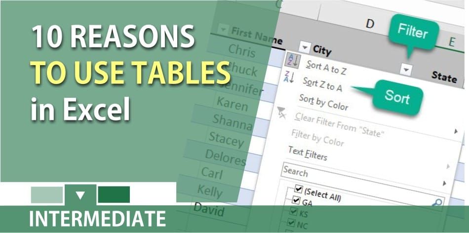
1. Filters
The first thing you’ll notice when you create a table is that filtering controls are added to the table headers automatically. To apply filters, simply click the drop-down arrow in the table header of the column you want to filter by. If you don’t want to see the filters, uncheck the box next to _Filter Button_ in the _Table Tools Design_ tab.

2. Sorting
You can use the filter arrows to sort data by any column quickly. To sort by multiple fields at a time, use Data Sort.
3. Easy Data Entry for Charts and PivotTables
If you have a chart created with a data range, and you add a new record in the row at the end of the range, the chart won’t pick up the added record, but if your data is in a table, adding a new record makes the table expand automatically to include the new record and your chart automatically updates.
Another awesome feature is that this also applies when you add data into a new column. With the months of January and February in B1 and C1 respectively, add March to D1 and your chart updates.
Do you use PivotTables? After adding records to your table, simply go update your PivotTable. With a data range, you would have to go to Change Data Source and include the new records.
4. Automatic AutoFill
In a table, when you add a new record, not only does the formatting extend but the table will also automatically AutoFill any formulas you have in your table. This is a great time saver.
**Promo video for** **free** **online course on tables**
Five Reasons to Use Tables in Excel by Chris Menard - Free Course - YouTube
5. Calculated Columns
This is one my personal favorites. Do you need to add a formula in a blank column? With tables, when you enter a formula into an empty column, Excel will use calculated columns to automatically fill in the rest of the rows in the column. This is much faster than AutoFill.
If you have 500,000 rows of data, calculated columns will also reduce errors. As mentioned in step 4, calculated columns will adjust and continue to add your formula as you add or delete records in the table.
More good news: if you need to edit the formula in a calculated column, simply edit the formula in one cell – it doesn’t matter which one, you could even be in the last cell of a column – and the change automatically applies to all rows.
6. Headers always available
With a data range, the header row will disappear when you scroll down your worksheet. When you create a table, the header row in the table is always visible without requiring the use of the Freeze Panes command on the View tab.
7. Total Row
Click anywhere in your table and under the Table Tool tab, check Total Row. You can now use functions with the drop down arrow in each cell in the total row.

8. Quick Formatting
You can use the Table Styles group under the Table Tools Design tab. This is one of the fastest ways to format your data. After picking a style, you can use Banded Rows and Banded Columns to change the look of your table style. You can use First Column and Last Column for more formatting options.
9. Automatic Naming
When you use a table and do calculations, names appear automatically.

10. Quick Totals
When you create a table, you can add a total row to your table, by clickingTotal Row in Table Tools Design. With the Total Row, you can perform a variety of Excel functions easily.