Create a data validation drop down list in Excel

You can use data validation to restrict the type of data or the values that users enter into a cell. An example would be if you have a column for Departments, and someone puts in Accounting but another person types in Acct. (abbreviating Accounting). Data validation keeps bad data from being entered. When bad data is entered into Excel, here are features that don’t work correctly:
1. Filters 2. Database functions 3. PivotTables 4. PivotCharts 5. Subtotals 6. Sorting 7. Advanced Filters
One of the most common data validation uses is to create a drop-down list. You can provide a more efficient worksheet by using drop-down lists in cells where people can make a Yes or No choice, or pick from another list you insert.
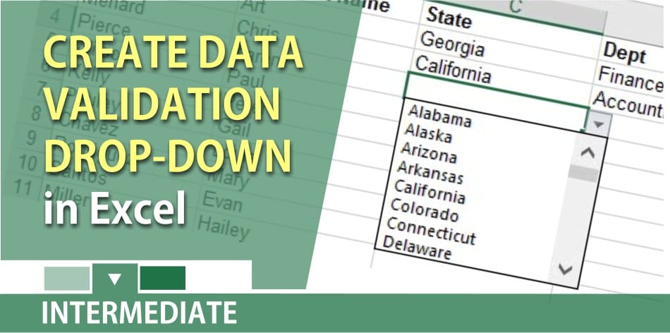
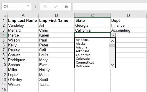
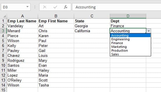
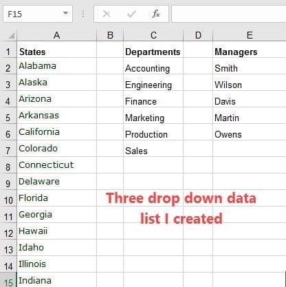
Someone using your worksheet clicks an arrow and then clicks an entry in the list. Below are examples of two drop-down lists I being used in the first two images, and image 3 shows the worksheet with the drop-down list. Click an image to enlarge it.
Image Gallery of Drop Down Validation List


Steps to create a drop-down list:
1. We are going to make a drop-down list for Departments in my example. Click in a blank worksheet. In cell **A1** type **Department**, press **Enter**, click back in A1 and make Department bold. 2. In **A2** type in Accounting. 3. In **A3** type in Finance. 4. In **A4** put in Marketing. 5. In **A5** put in Sales 6. Now select **A2 to A5**. 7. Click the **name box** and type in **DEPT** and press **Enter**. You just named A2:A5 DEPT. In the next section, we will use the list.
How to use the drop-down list you created
1. Click on a new worksheet. How we are going to use the drop-down list we created. In **A1** type in the **Last Name**, in **B1** type in **First Name**, and in **C1** type in **Department**. Widen the columns if necessary. 2. Select A1 to C1 and make Bold. It is your header row. To save time assume that last names and first names are in column A and column B respectively. 3. Select **C2 to C15**. 4. Click the **Data** tab and click **Data Validation** under the data tools group. 5. By default, it read Any Value. Click the drop-down arrow and select **List**. 6. In the Source box type **=DEPT** and click **OK** 7. Click in cell C2 and use the drop-down arrow. 8. Click in C3 and type in **Acct** and press **Enter**. You will get an error message because Acct is not a department.
YouTube video on creating a drop-down list
Create a data validation list in Excel by Chris Menard


