Count Unique Values in Excel with UNIQUE, SORT, and COUNTIF Functions Tutorial

Table of Contents

• 📋 Why this method works and when I use it
• 📋 Setting up the table
• 🔎 Extract distinct values with UNIQUE
• ↕️ Sort the unique list with SORT
• 🔢 Count occurrences using COUNTIF
• ✅ Why tables beat ranges for this task
• 🔁 When to use this instead of a pivot table
• 🔧 Quick checklist to implement this
• ❓ Frequently asked questions
• 📌 Final tips

📋 Why this method works and when I use it

I often need a quick way to show how many times each item appears in a column without building a pivot table. Using the UNIQUE, SORT, and COUNTIF functions together gives me a dynamic, easy-to-share result that updates automatically when my data changes—provided the data is in an Excel table.

This approach is especially useful when I’m sharing a workbook with someone who might not know how to refresh a pivot table. A simple formula-driven summary stays live and accurate for anyone who uses the file.

📋 Setting up the table

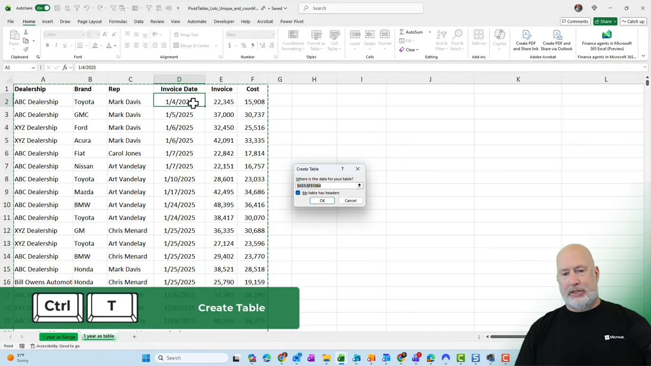
The first thing I do is convert my raw data into an Excel table. Select any cell in the data and press Ctrl+T. Make sure the header row is selected. In my example, I had 1,063 records and a column for car brands.

I prefer tables because they expand automatically when you add rows. That means formulas that reference the table will pick up new records without having to adjust ranges manually.

,

🔎 Extract distinct values with UNIQUE

Once the data is formatted as a table, I extract the distinct items with UNIQUE. If my table is named Table2 and the brand column is Table2[Brand], the formula I use is:

=UNIQUE(Table2[Brand])

I put that formula where I want the list of brands to appear. Because UNIQUE spills its results into adjacent cells, it will dynamically return every distinct brand and grow or shrink as the source data changes.

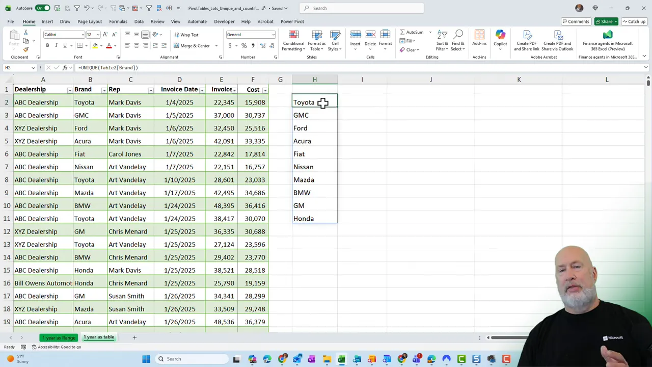
↕️ Sort the unique list with SORT

I like my summaries sorted alphabetically or in a specific order so they are easier to scan. You can wrap UNIQUE inside SORT like this:

=SORT(UNIQUE(Table2[Brand]))

That returns a neatly ordered column of brand names. Sorting is optional, but it improves readability when you share the workbook with others.

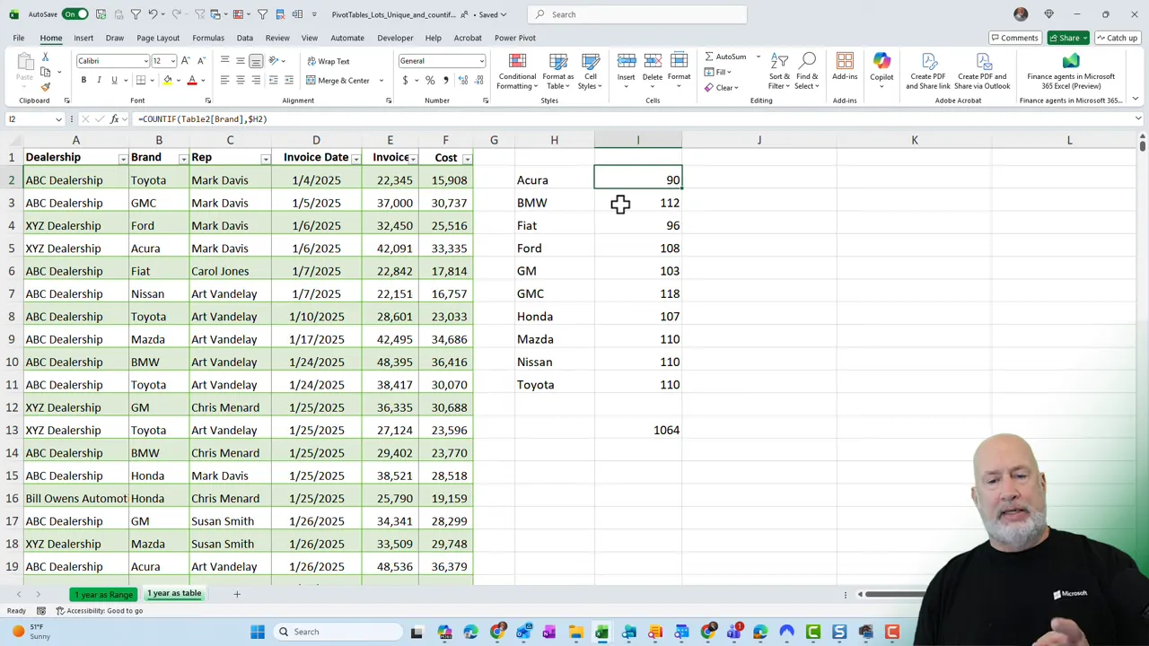
🔢 Count occurrences using COUNTIF

Now for the counts. I place a COUNTIF next to each unique brand to calculate how many times it appears in the source column. The pattern looks like:

=COUNTIF(Table2[Brand], H2)

Where H2 is the cell containing the brand you want to count, I often use a mixed reference by locking the column of the unique list while leaving the row relative so that I can drag the formula down. This is a personal preference and not required for the formulas to work.

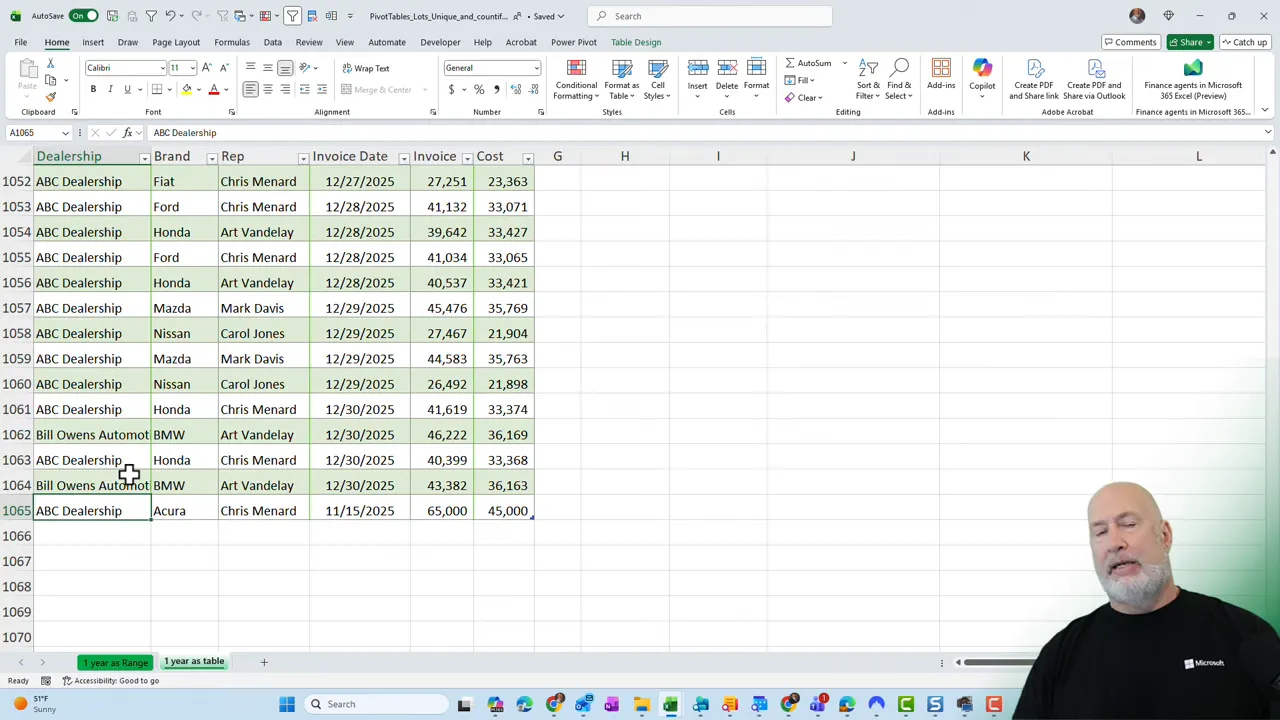
To verify totals, I use an AutoSum at the bottom and ensure the sum equals the total number of records. In my example, I had 1,063 records, and the sum of the counts matched that number.

✅ Why tables beat ranges for this task

The main advantage of using a table instead of a plain range is automatic expansion. If you type a new row at the bottom or paste data into the next row, the table picks it up. The UNIQUE and COUNTIF formulas that reference the table will update immediately.

If you use a non-table range, adding rows does not automatically extend the named range or cell references. That means your summary formulas will not include the new data unless you manually change the ranges.

I demonstrate this by adding a single record to my table and seeing the count for that brand increase immediately. That immediate update is the difference between a reliable, shareable spreadsheet and one that requires constant maintenance.

🔁 When to use this instead of a pivot table

Pivot tables are powerful and often the right tool for summarizing data. They also offer automatic refresh in recent versions of Excel. However, I choose the UNIQUE + SORT + COUNTIF method when:

• Someone who will use the file might not know how to refresh a pivot table.
• I want the summary to update instantly as data is added to the table.
• I need a simple, formula-based layout that’s easy to edit or format inline.

If you know your audience is comfortable with pivot tables and you want advanced summarization features, a pivot table may be the better choice. But for automatic, always-up-to-date counts that require no manual refresh, formulas in a table are hard to beat.

🔧 Quick checklist to implement this

1. Create a table with Ctrl+T.
2. Use =SORT(UNIQUE(TableName[Column])) to list distinct values in order.
3. Use =COUNTIF(TableName[Column], CellWithUniqueValue) next to the list.
4. Confirm the sum of counts matches your total records.
5. Add rows to the table and watch the summary update automatically.

❓ Frequently asked questions

How do I extract unique values from a column?

Use the UNIQUE function on the table column or range. For example: =UNIQUE(Table2[Brand]). If you want them sorted, wrap UNIQUE with SORT: =SORT(UNIQUE(Table2[Brand])).

Why should I convert my data to a table first?

Tables expand automatically when you add rows. Formulas referencing table columns will automatically include new records, keeping UNIQUE and COUNTIF results accurate as the dataset grows.

Can I use COUNTIFS instead of COUNTIF?

Yes. COUNTIFS is helpful if you need multiple criteria. For a single-column count per unique value, COUNTIF is simpler and faster: =COUNTIF(Table2[Brand], H2). Use COUNTIFS when you must filter by additional columns, such as date or region.

When should I use a pivot table instead?

Use pivot tables for multi-field analysis, grouping, and built-in layout options. Choose formulas when you want a lightweight, always-updating summary that anyone can open without refreshing a pivot table.

How do I ensure the formulas remain readable for others?

Use named tables and clear column headers, place the unique list and counts beside the table, and add a short note explaining the formulas. That makes the workbook self-documenting and easier to hand off.

📌 Final tips

Keep the formulas simple and rely on tables for robust behavior. Small touches like sorting the unique list and verifying totals help prevent errors and make the results easier to consume. When in doubt, choose the method that keeps your audience in mind: formula-based summaries for ease and reliability, pivot tables for power and flexibility.